|
The solution of
a DP model is found with the DP Solver add-in (dp_solver.xla).
This program can be run independently, but the easiest way
to use it is to construct a model with the DP Models add-in
and call the DP Solver from the model page. Click the Transfer
to DP Solver at
the top of the model page. |
| |
|
Three kinds of DP Solver models are available. The first, Transition
List, presents the data much like the lists constructed
by the DP Models add-in. All transition information is
described by lists. The number of transitions determines
the number of rows in the Solver model. Excel allows
very many worksheet rows.
The second option, Probability/Cost Matrix, shows
the transition probabilities and costs as matrices. The
dimensions of the two matrices are (number of decisions)x(number
of states). For small problems this is the most visual
representation. For larger problems, the problem size is
limited by the number Excel columns. With older versions
of Excel the number of columns restricts the use of this
representation to about 100 states. Excel 2007 allows many
more worksheet columns than Excel 2003, thus increasing
the problem size. Viewing the transition matrix is not
very useful for large problems because the nonzero transitions
are usually a very small proportion of the total number
of matrix entries.
The third format, Probability/No Cost Matrix,
shows the transition probabilities as a matrix, but computes
the expected transition cost and shows that result in a
single column. Models of this form are limited to about
200 states.
For this example we use the Transition List option.
The same DP model can
provide the data for several Solver worksheets by entering
different names in the name field.
|
|
| |
The DP Solver model
has much the same appearance as the lists created by the DP Models
add-in. The primary differences are columns created for computation
of solutions. Data is simply copied from the lists rather than
linked through formulas. If the model changes the DP Solver form
must be rebuilt. The user need not interact with DP Solver
form. All equations are automatically inserted and solutions
are obtained by clicking Solve button at the top of
the worksheet. |
Parameters |
|
 |
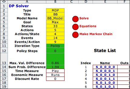
The DP Solver
model is placed on a new worksheet called BB_DP. Parameters
are placed at the upper left corner of the worksheets. Yellow
cells hold parameters that should not be changed. The green
cells hold information about the current DP solution technique
employed. Important to this discussion are the two cells labeled Maximum
Value Difference and Sum Probability Difference.
The values in these cells should converge to zero as the algorithm
progresses.
|
States |
| |
Columns D through J hold
data for the states of the model. The yellow cells in the figure
below hold equations provided by the add-in. Columns that participate
in the solution process are the State Value (Column
Q) and the Next Value (column R). The goal of this optimization
is to find the action for each state that maximizes the State
Value. In this case the state value is the number of runs produced
during an inning of play. An iterative process finds the optimum
action for each state. They are represented in the table below
by the Action
Index column
and the Action
Name column. The iterative dynamic program terminates when
the State Value and Next Value are
close enough. This is indicated by the Maximum Value Difference that
is computed as the maximum absolute value difference between
the State Value and Next Value. The
iterative process also determines the state probabilities for
the optimum policy. These are computed in columns S and T. They
aren't very interesting for this example since the process always
terminates in the final state. |
|
| |
The values shown in columns
Q through T are the initial values. We will see that these
values converge to the optimum values after the application of
dynamic programming. |
Actions and Events |
| |
|
The actions and event definitions are transported
to the DP Solver model as shown on the left. The columns
labeled Runs and Probabilities are irrelevant
for this example. The number of runs and the probabilities
of transition are not a function of either the action or
event alone. Run production depends in a complex way on
the state, action and event. The probability of a transition
depends on the action and event. These are all defined
in the transition blocks discussed below. |
|
Decisions |
| |
The first six columns
of the decision list are copied from the model. Columns AM through
AP compute values necessary for optimization. Only 34 of the
decisions are shown. There are 78 decisions for this problem,
each characterized by a state and an action. |
| |
|
Transitions |
| |
There are 402 transitions described
for this problem. A few are shown on the transition list below.
Most of the data is copied directly from the model lists.
The final two columns are important for computing the results
of the DP. |
|
Optimization |
| |
 |
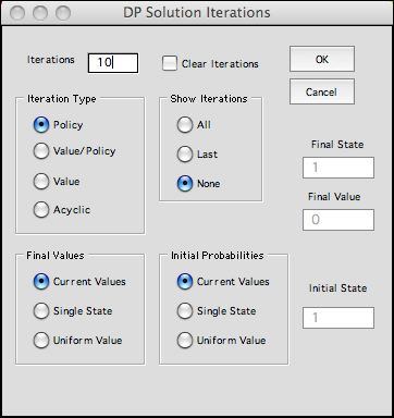
We solve the DP by clicking on the Solve button
at the top of the page. There are several solution options.
We choose
to solve the DP with the Policy method. This finds
the optimum policy in one step. The results are shown below. |
|
| |
The optimum action
is found for each state. It happens for this data that the
optimum solution is the Hit action, no matter what the
state. Although this seems like an uninteresting policy, it is
one that couldn't be determined without this kind of analysis. |
|
| |
An interesting result is the State
Value for the initial state (0,0,0,0), no outs and no
one on base. The value is 0.8122. That is the expected run
production in the inning when the optimum policy is followed. |
Alternative Data |
| |
 |
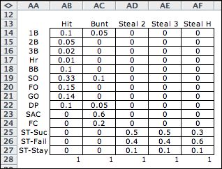
To illustrate the flexibility of the DP
Models add-in with different data, we change the data table
to represent a player with less power but more speed. The
new data is shown at the left. The new solution is shown
below.
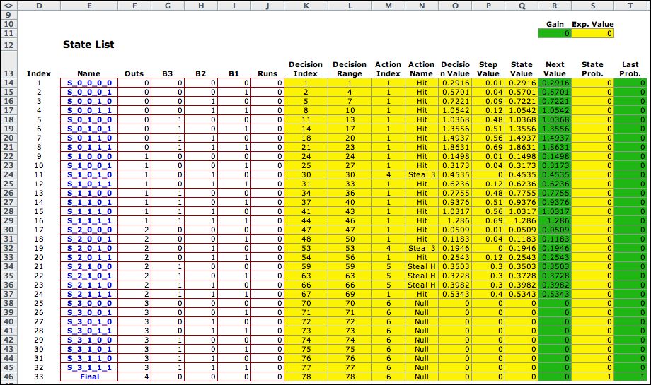
The solution describes a policy that involves more base
stealing. The expected runs in the inning with this policy
is reduced to 0.2916 runs per inning. The faster team has
a different strategy but with less scoring. |
|

|
Modifications |
| |
The model involved a single inning
with one kind of player. The rules of baseball were followed,
but not all the events were accurately modeled. The biggest
assumption is that all batters and runners have equal
skills. It would be interesting to describe a batting order
for the inning so that each player had a different action/event
probability matrix. Assuming a nine place batting order, the
model would be at least nine times the size of this model,
but it would fit the Excel worksheet. No attempt has been made
to model or solve the larger problem. |
| |
|


