|
This
example comes from a book Introduction to Stochastic Programming by
Sheldon M. Ross, (Academic Press, 1982). In the book the problem
is described with a continuous nonnegative state unbounded
from above. The action variable is also continuous. For our
purposes we will discretize both state and action.
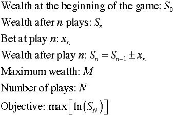
A gambler is playing a game that
has two results, win or lose. He can bet any amount up
to his entire wealth. If he wins the amount of the bet
is added to his wealth, and if he loses the amount of
the bet is subtracted from his wealth. The gambler's
goal is to maximize the log of his wealth after a fixed
number of plays. |
To make analysis possible, we define the gambler's wealth
as the state variable measured in whole dollars. We restrict
the gambler's wealth to be less than the quantity M.
Bets are measured in dollars and in this model the
amount of the bet is the action variable. Bets
are restricted so that the gambler can never bet an amount
that would reduce his wealth to less than $1 or more than M.
There are N plays in the game and the objective is
to maximize the log of the wealth after play N.
|
States |
| |
The states are defined
with a single state variable. The
state definition region on the model worksheet is shown below.
Cell F14 holds the value of the current state, 10. For the
example we choose to limit the wealth to $20. The lower bound
on the state is in F18, and the upper bound is in F19.
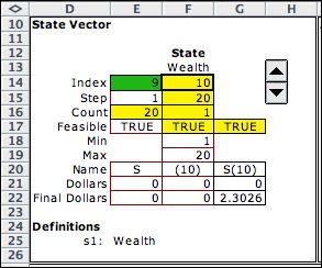
The example illustrates a new feature of the DP
Models add-in, the ability to define the values for the final
state. This is important for finite time horizon problems. For
the Gambler problem, the only objective concerns the value at
the final state. The goal is to maximize the log of the wealth
at the end of the time horizon, 20 plays for the example shown
above.
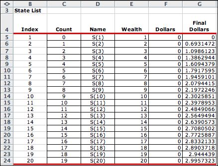
After enumeration the state list appears as below.
The Final Dollars column is computed as ln(final wealth).
|
Actions |
| |
The action is the
amount the gambler bets on a given play. The range of bets is
defined in the action element. The goal of the DP is to select
bets at each state to maximize the log of the wealth at the end
of the game. |
|
|
Events |
| |
The event indicates whether
the bet wins or loses. The probability of winning is a parameter
of the system, stored in Q24. The example assumes the probability
of winning is 0.6 with a corresponding probability of losing
of 0.4. The summary starting in column S shows that the combination
of elements, S(10)/Bet(5)/Win, is feasible. |
|
Decisions |
| |
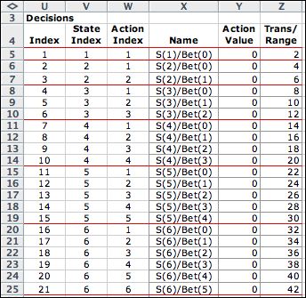
Not all combinations
of state and action are admissible. We reject all actions that
might lead to a state less than 1 or more than 20. This is accomplished
in the single decision block of the model. The Max entry
in column K holds a formula that limits the size of the bet.
The maximum bet with a wealth of 10 is a bet of 9. any larger
bet allows the possibility that the wealth falls below 1 or above
20. |
 |
| |
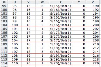
Enumeration of the elements
reveals that there are 110 feasible combinations of state and
action. Near the top of the list the actions are limited by the
risk of falling below 1. Near the bottom of the list the actions
are limited by the possibility of falling above the maximum wealth
of 20. |
| |
.
|
Transitions |
| |
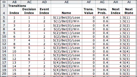
The transition equation
is particularly simple for this model. The change state cell,
F64, contains a formula that evaluates the positive of the bet
for a win event, and evaluates as the negative of the bet for
the lose event. The example shows that betting 5 when the wealth is
10 increases the wealth to 15 because of the win event. |
 |
| |
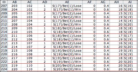
There are two events
for every decision so the transition list has 220 entries. |
| |
.
|
| |
The gambler problem is
solved on the next page. |
| |
|


