|
|
Another classic problem that can be modeled as a linear program
concerns blending or mixing ingredients to obtain a product
with certain characteristics or properties. We illustrate this
class with the problem of determining the optimum amounts of
three ingredients to include in an animal feed mix. The final
product must satisfy several nutrient restrictions. The possible
ingredients, their nutritive contents (in kilograms of nutrient
per kilograms of ingredient) and the unit cost are shown in
the following table.
The mixture must meet the following restrictions:
- Calcium — at least 0.8% but not more than 1.2%.
- Protein — at least 22%.
- Fiber — at most 5%.
The problem is to find the composition of the feed mix that satisfies
these constraints while minimizing cost.
|
Nutritive content and price of ingredients
|
|
Ingredient
|
Calcium
(kg/kg)
|
Protein
(kg/kg)
|
Fiber
(kg/kg)
|
Unit cost
(cents/kg)
|
|
Limestone
|
0.38
|
0.0
|
0.0
|
10.0
|
|
Corn
|
0.001
|
0.09
|
0.02
|
30.5
|
|
Soybean meal
|
0.002
|
0.50
|
0.08
|
90.0
|
|
|
| |
Variable Definitions
L, C, S : proportions
of limestone, corn, and soybean meal, respectively, in the
mixture.
Constraints
The number of hours available on each machine type is 40 times
the number of machines. All the constraints are dimensioned
in hours. For machine 1, for example, we have 40 hrs/machine ¥ 4
machines = 160 hrs. In writing out the constraints, it is customary
to provide a column in the model for each variable.
|
Minimum calcium: |
0.38L |
+ 0.001C |
+ 0.002S |
> 0.008 |
|
Maximum calcium: |
0.38L |
+ 0.001C |
+ 0.002S |
< 0.012 |
|
Minimum protein: |
|
+ 0.09C |
+ 0.50S |
> 0.22 |
|
Maximum fiber: |
|
+ 0.02C |
+ 0.08S |
< 0.05 |
|
Conservation: |
L
|
+ C |
+ S |
= 1 |
Nonnegativity
L, C, S > 0
Objective Function
Because each decision variable is defined as a fraction of
a kilogram, the objective is to minimize the cost of providing
one kilogram of feed mix.
Minimize Z = 10L + 30.5C +
90S |
|
| |
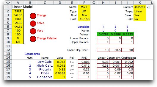
The model was created by the Math
Programming add-in and solved with the Jensen LP/IP Solver.
The solution shows the optimum proportion
of each component of the feed. The objective value is the cost
per kilogram of the minimum cost mix that meets the nutruitive
requirements. 
Sensitivity Analysis
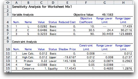
The sensitivity analysis created by the Jensen Solver shows
that the upper bound of the calcium constraint and the lower
bound of the protein constraint are limiting the solution.
The shadow prices are the derviatives of the unit cost of
the feed with respect to the tight bounds. For example, if
one increases the upper bound of the calcium constraint from
0.012 to 0.013 the cost will be reduced by about $0.20.
cost increase = shadow price * bound increase
= (-19.62)(0.001) = -0.1952.
In like manner, if the lower bound on protein
were increased from 0.22 to 0.23 the cost would be increased
by about $1.45.
cost increase = shadow price * bound increase
= (145.17)(0.01) = 1.4517.
The fiber constraint is strictly between its
bounds, so the shadow price is zero. 
|
|