Find the optimum product mix

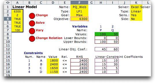
The problem is to find values of P and Q that maximize the objective of the problem. We use the Mathematical Programming add-in to generate the model in Excel. The model is then solved with the Excel Solver. The worksheet with the model is shown below. Notice that the model has four constraints representing the machine times. The market constraints on production are represented as simple upper bounds. These could have been included in the constraint set, but using simple upper bounds provides a more compact model.

The solution is shown under P and Q in row 8. The optimum solution is to produce 100 units of P and 30 units of Q.

The net profit of this solution is $300. That is the $6300 shown in cell F4 on the worksheet, less the $6000 operating expense. The latter was not included in the model because it does not affect the optimum decisions. Constant values are never included in the objective function.

Find the bottlenecks

Find the range over which the unit profit may change

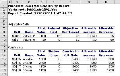
This result is determined from the sensitivity analysis. We show below the sensitivity analysis created by the Excel Solver. The part of the analysis labeled Adjustable Cells provides information concerning the variables and the objective function. Each row on this table represents a variable. The Cell entry is the Excel reference to the cell holding the variable value for the optimum solution. The Name is provided by the name appearing above the value cell on the model worksheet (row 7). The Final Value is the amount of that variable for the optimum solution. The Reduced Cost is the change in the optimum objective per unit change in the upper or lower bounds of the variable. Since the final value of P is equal to the simple upper bound, the reduced cost tells us that the objective function will increase by 15 per unit increase of that upper bound (100). Neither the upper or lower bound for Q is restricting, so its reduced cost is 0. The reduced cost really represents a derivative of the objective function with respect to the variable bound. It may be true that a unit change cannot be made without some other constraint becoming tight.

The Objective Coefficient column provides the current value of the objective coefficient. The next two columns tell how much that coefficient can change before the optimum solution changes. We see that the Allowable Increase in the objective coefficient for P is essentially infinity and the Allowable Decrease is 15. This means that the unit profit (objective coefficient) can range between 30 and infinity while the current solution ( P=100 and Q = 30) remains optimal. The unit profit of Q can range between 0 and 90 with the current solution remaining optimal. It should be emphasized that these ranges are correct only if one profit coefficient is changed at a time.

Find the marginal benefit of increasing the time availability

The part of the sensitivity analysis labeled Constraints, gives information concerning changes in the constraint right-hand sides. Each constraint provides a row on this table. The Cell entry is the Excel reference to the cell holding the constraint value. The Name is provided by the name to the left of the value cell on the model worksheet (column C). The Final Value is the amount of the constrained quantity used by the optimum solution. In this case it is the machine time used.

The column labeled Shadow Price gives the marginal benefits of increasing the time availability. For machines A, C and D the marginal benefit is zero. Since these machines are underutilized, there is obviously no benefit for providing additional minutes.

The shadow price for machine B is 2. This means that an extra minute of machine time yields an increase in profit of $2. This number is valid throughout the range indicated by the last two columns. That is, for product B, the shadow price of 2 is valid for any availability between 1500 and 3000 minutes.

Find the range over which the time availability may change

The Allowable Increase and Decrease columns give the change in the constraint limit within which the current basis remains optimal. This means the bottlenecks remain the same in this range.

We learn from the row for A that the machine availability can go as low as 1800 and as high as infinity. Of course this is reasonable because this constraint is loose with 600 unused minutes for the machine. Similar comments can be made about machines C and D.

The range for machine B is from 1500 to 3000 minutes. Since this constraint is tight for the optimum solution, certainly as the time available for B changes, the amounts of products P and Q must change. The interesting result is that the time on machine B and the market for P remain the bottlenecks within the range.

Parametric Analysis

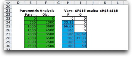
The Vary button on the worksheet provides a parametric analysis where a single number is varied over a range and the optimum reported for several values. For the example, the time available for machine B is an important parameter, so we vary that value from 0 to 3500 minutes in steps of 500 minutes with the following results.

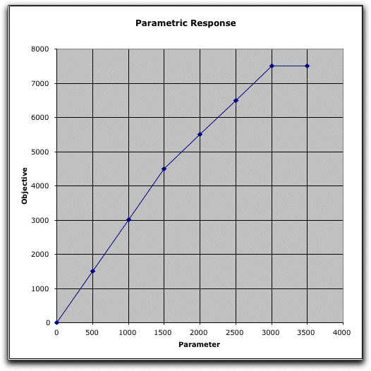
The add-in provides a graph of the objective as a function of the parameter. The limits observed in the sensitivity analysis for the right-hand side of the second constraint are clearly evident in the results. Below 1500, the variable P is basic, while Q is not. In the range 1500-3000, the variable Q is basic, while P is non-basic at its upper bound. Neither P nor Q is basic above 3000. Both are non-basic variables at their upper bounds.