Return to Index
Operations Research Models and Methods
 
Models Section


Models
Workforce Scheduling Problem


Workforce Scheduling Problem
Statement
Consider a bus company scheduling drivers for its buses. The requirement for buses varies from hour to hour because of customer demand as shown in the figure. Time 0 on the figure represents midnight, and times are shown with a 24 hour clock starting at midnight. For example, four buses must run from midnight to 4 a.m., while eight buses must run from 4 a.m. until 8 a.m. We assume that the bus requirements are the same every day.

The problem is to determine how many drivers to schedule at each starting time to cover the requirements for buses. Drivers work eight hour shifts that start at times: 0, 4, 8, 12, 16 or 20. For example, a driver starting at time 0 can drive a bus from time 0 to 8. A driver scheduled to start at time 20 works for the final four hours of the day and the first four hours of the next day. The goal is to minimize the number of drivers used. Note that although a driver can be hired for an eight hour period, there is no requirement that he drive a bus for the entire period. He might be idle for a four hour interval within the period.

One feasible solution to this problem is to schedule 8 drivers at time 0, 10 drivers at time 8, and 12 drivers at time 16. This solution will cover all the requirements and use a total of 30 drivers. The problem is to find the smallest number of drivers.
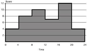
Requirements for buses in a 24 hour period


Model

  Variable Definitions

x(t) : Number of drivers scheduled at time t, t = 0, 4, 8, 12, 16, 20

We assume that this problem continues over an indefinite number of days with the same bus requirements and that x(t) is the number used in every day at time t.

Constraints

We need constraints that assure that the drivers scheduled at the times that cover the requirements of a particular interval sum to the number required. For the interval from time 0 to 4, drivers starting at time 20 of the previous day and time 0 of the current day cover the needs from time 0 to time 4. Then we write

The remaining constraints are:

The objective is to


Excel Model and Solution


Using the Math Programming add-in we create the model in Excel as shown below. The model has been solved using the Jensen LP/IP Solver.

The solution found by the linear programming algorithm (shown below) uses the minimum number of 26 drivers to meet the schedule. There are alternative solutions to this problem that can be found by observation.

Optimum Solution

x0

x4

x8

x12

x16

x20

Z

4

10

0

8

4

0

26

Sensitivity Analysis

The LP/IP Solver presents the sensitivity analysis below.

Since the objective function does not admit variation of its coefficients, the sensitivity analysis of the objective coefficients has no meaning in this context.

A tabular presentation of the constraint analysis is shown below. The constraint analysis identifies periods 4 and 12 with excess drivers. An additional unit of demand can be handled in these periods and also period 20 with no additional drivers. Period 20 is interesting because an increase in demand of 1 in that period can be met by scheduling one more driver to arrive at hour 16, and one less to arrive at hour 12. The solution does not provide this information, but the dual variable indicates that one more unit of demand can be met with no additional cost.

Constraint Analysis


D0

D4

D8

D12

D16

D20

Slack

0

6

0

1

0

0

Dual Value

1

0

1

0

1

0

Lower b

0

---

4

---

11

0

Current b

4

8

10

7

12

4

Upper b

---

14

---

8

---

5


Algebraic Model


The model below is more general than the example of this page in that it defines variables representing patterns of work. A pattern provides a worker for one or more periods, that may or may not be adjacent. We could identify the periods as hours in a day and each pattern would cover a specified set of hours.

The model can also be written in a more concise matrix format.

For the specific example addressed on this page, the components of the matrices are assigned numeric values.

Although we include this model in the section on linear programming, it is often reasonable to place the requirement of integrality on the decision variables x. Clearly it is impractical to schedule fractions of workers. In general it is much more difficult to solve linear problems with the addition of the integrality requirement than without. Unless it is crucial to the usefulness of a solution we will not require integrality. We consider integer models in a later section.


Return to Top

tree roots

Operations Research Models and Methods
Internet
by Paul A. Jensen
Copyright 2004 - All rights reserved