A typical transportation problem is shown in Fig. 9. It deals with sources where a supply of some commodity is available and destinations where the commodity is demanded. The classic statement of the transportation problem uses a matrix with the rows representing sources and columns representing destinations. The algorithms for solving the problem are based on this matrix representation. The costs of shipping from sources to destinations are indicated by the entries in the matrix. If shipment is impossible between a given source and destination, a large cost of M is entered. This discourages the solution from using such cells. Supplies and demands are shown along the margins of the matrix. As in the example, the classic transportation problem has total supply equal to total demand.

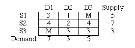
Figure 9. Matrix model of a transportation problem.

The network model of the transportation problem is shown in Fig. 10. Sources are identified as the nodes on the left and destinations on the right. Allowable shipping links are shown as arcs, while disallowed links are not included.

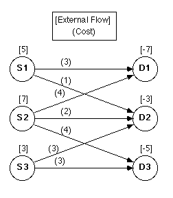
Figure 10. Network flow model of the transportation problem.

Only arc costs are shown in the network model, as these are the only relevant parameters. All other parameters are set to the default values. The network has a special form important in graph theory; it is called a bipartite network since the nodes can be divided into two parts with all arcs going from one part to the other.

On each supply node the positive external flow indicates supply flow entering the network. On each destination node a demand is a negative fixed external flow indicating that this amount must leave the network. The optimum solution for the example is shown in Fig. 11.

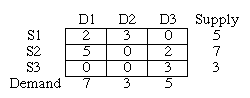
Figure 11. Optimum solution, z = 46.

Variations of the classical transportation problem are easily handled by modifications of the network model. If links have finite capacity, the arc upper bounds can be made finite. If supplies represent raw materials that are transformed into products at the sources and the demands are in units of product, the gain factors can be used to represent transformation efficiency at each source. If some minimal flow is required in certain links, arc lower bounds can be set to nonzero values.