|
|
 |
Random
Variables |
 |
-
Stochastic Programming |
 |
Stochastic programming
concerns mathematical programming models where some parameters
are uncertain. Rather than deterministic numbers, these parameters
are described as random variables. For stochastic programming,
some variables are to be set by a decision maker, these are
the decision variables, while some model parameters are determined
by chance, these are the random variables.
There are a variety of situations one might consider in this
context. One differentiation is based on when the decision maker
must make decisions relative to the time when the random variables
are realized. There are several possibilities.
No Recourse: The decision maker must choose values for the
decision variables before any of the random variables are
realized.
Single Stage Recourse: Some of the decision variables must
be set before the random variables are realized, while others
may wait until after they are realized.
Multistage Recourse: Decisions and random variables are determined
in stages. The first set of decision variables must be fixed
before all realizations. Then the first set of random variables
are realized and the second set of decision variables must
be fixed. The process continues through a series of decisions
and realizations. Typically the stages represent intervals
of time.
Wait and See: The decision maker makes no decisions until
all random variables are realized.
Of course, the decision maker prefers the last case. Then the
optimum decisions can be made with no uncertainty using a deterministic
optimization procedure. The first case is the most difficult
because the all decisions must be made before the model is completely
known. It is not obvious how decisions should be made in this
case, but we investigate some alternatives below using the Algorithm
feature of the add-in.
We consider on this page the first and last cases since for
these the Function feature of the add-in provides useful
information. The cases that involve recourse are the subject
of much active research. This subject is beyond this simple
introduction, but we consider an example on the next page. |
Wait and See |
| |
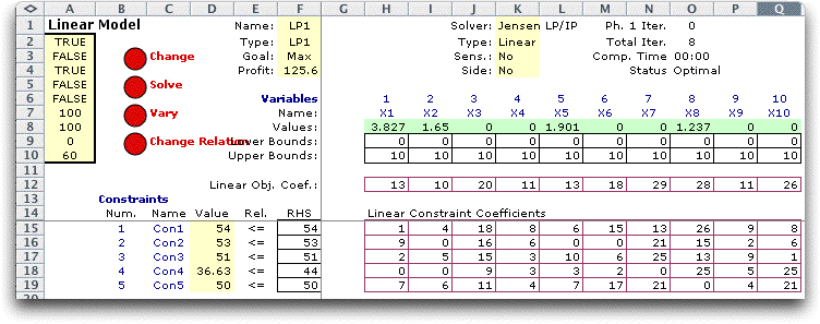
To illustrate stochastic programming,
consider the linear programming model below. The solution algorithm
is the Jensen LP/IP add-in. The problem was generated randomly
using the Math Programming add-in. The solution shown is the optimum
solution when all parameters of the model are deterministic. |
 |
| |
For this situation we assume that
the RHS vector (F15:F19) is uncertain. In particular, we assume
that the RHS values have the mean values as given, but the values
have Normal distributions with given standard deviations. To create
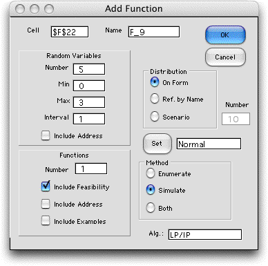
a stochastic model, we choose Function from the menu
and fill in the dialog as below. We have specified LP/IP as the
algorithm. This means that the LP will be solved for each point
of the sample space that is generated by the enumeration or simulation
procedure. For the example we use simulation. |
| |
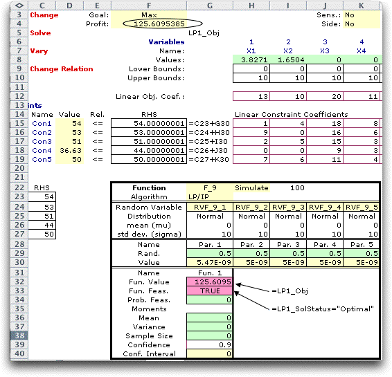
The form is placed below the LP model as shown
below. The figure shows some of the modifications required
for the analysis. The RHS entries shown in column F have been
replaced by the equations in column G (the equations are placed
in column F, but illustrated in G). Each RHS is the sum of
the original value stored in column C and a Normally distributed
random variable defined on the simulation form. The random
variables all have a mean of 0 and a standard deviation of
10. The function value in G32 is an equation that links to
the LP objective in F4. The feasibility value in G33 is a
logical statement that points to cell O4 (shown with the LP
model above). That cell, filled by the LP/IP add-in, holds
the word "Optimal" only when the model has a feasible
solution. The particular solution shown has all random variables
set to 0, their expected values.
|
|
| |
This form illustrates
a case where important features of the stochastic model lie
in the portion of the worksheet outside the form. The random
variables are linked by equations to the RHS cells, and the
function value and feasibility state are linked by equations
to cells computing the objective function value and optimality
state.
To simulate the model choose Moments from
the menu and set the number of simulation observations to 100.
The results start in row 34 of the figure below. The numbers
shown in rows 29 through 33 are for the final simulated observation
of the random variables.
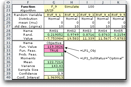
Even though the solution is optimum for each simulated
RHS, the mean objective function (estimated at 122.7 in cell
G36) is lower than the value when the RHS values were set to
their expected values (125.6). This is a consequence of "Jensen's
Inequality" (named after a different person that the author).
The expected value solution will always have a higher objective
function (when maximizing) than a solution that explicitly represents
uncertainty.
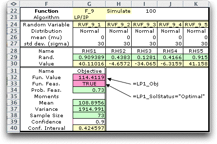
All the observations in the sample of 100 were feasible
for the example above. It is interesting to increase the standard
deviation of the random variables to 30, thus increasing the
variability of the RHS values. The simulated results are below.
For this model, the solution is infeasible only if one of the
RHS values is negative. With the data provided, the proportion
of feasible solutions is 0.73. The mean objective value is decreased
with significantly greater variance over the case when the standard
deviation values were 10. There is a price to pay for variability,
even with the wait and see policy.
|
|
No Recourse |
| |
With the no recourse situation,
we must fix the decision variables before the random variables
are realized. We might ask how well the expected value solution
serves as the solution to this problem. We create a different
model below. The LP model is the same as before, but now we
allow the RHS values to vary randomly but do not solve the LP
for each sample. For each sample, the solution is fixed at the
deterministic solution obtained with the expected RHS. The objective
value does not change because the decision vector is fixed.
The only question is what is the probability that this solution
will be feasible?
We have placed logical expressions in column G to indicate
when the constraints are feasible. The logical expression for
feasibility in cell G33 is TRUE only when all constraints are
all satisfied. The LP solution that is partially shown is optimal
when the RHS takes the expected value, so this solution is feasible.

When we simulate the model for this case we do not solve the
model for every sample. The word "None" in cell G23
assures this. The results are shown below. The objective value
shows no variability since the decision variables remain the
same for all samples. The proportion of feasible solutions is,
however, only 6%. The probability that this fixed solution is
feasible is very small.
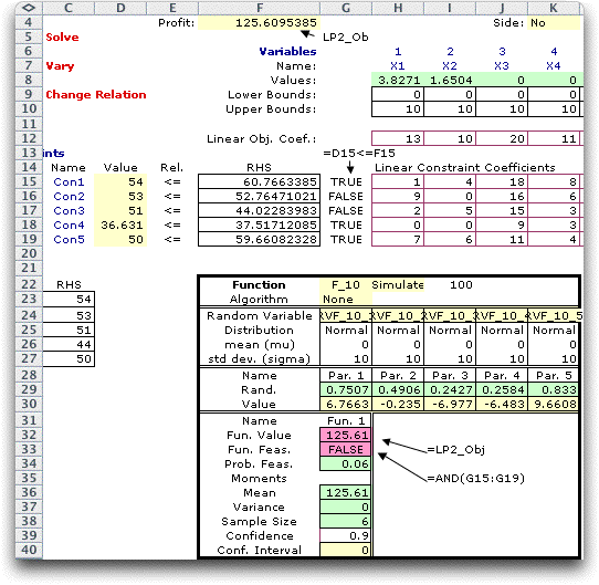
These results should not be surprising. With the
expected RHS values, four of the five constraints are tight
in the deterministic optimal solution. Since the RHS values
are normally distributed, there is a 50% that a tight constraint
will be violated when the random RHS is realized. Even if the
single loose constraint is never violated, the probability that
all the tight constraints are satisfied is 0.5 raised to the
fourth power or 0.0625. The simulated result is quite close
to this value.
One might ask, how should this problem be solved?
The answer to this question is part of the subject of stochastic
programming. |
Chance Constrained Programming |
| |
One way to find a solution that
has a greater feasibility probability is to make the RHS vector
smaller and solve the deterministic problem. A smaller RHS provides
a greater probability that a constraint will be satisfied for
a sample RHS. Say we set the RHS values so that there is only
a 10% probability of violating each constraint individually.
This is easily accomplished by setting the values in row 29
to 0.1. The values of the random variables in row 30 are values
that have a 90% chance of being exceeded. The solution shown
is optimal for the RHS values shown. The objective value is
94.6.
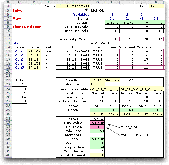
The results shown starting at row 34 are for a
simulation of 100 sample points. Even though each constraint
has a 90% probability of violation, the probability that all
constraints are feasible (the solution is feasible) is approximately
54%. |
Combining Wait and See Solutions |
| |
One suggestion often made for this
kind of problem is to solve the problem as if we could wait
and see the random realizations and then combine the wait and
see decisions in some way. We do this for the example by creating
a new math programming model identical to the wait and see model
considered earlier, but create a simulation form that records
the values of the decision variables as well as the objective.
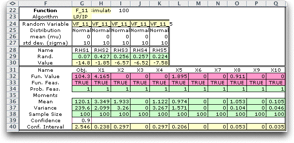
The form is below. We now have 11 functions defined. The first
is the objective function and the remaining ten are the values
of the decision variables. All eleven functions have the same
feasibility equation.
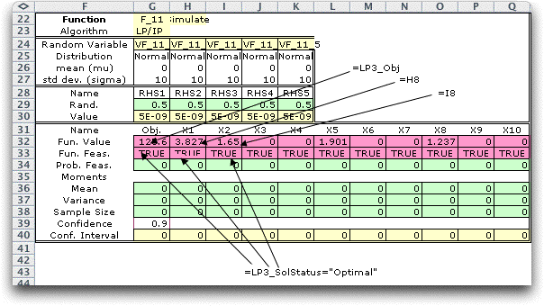
We simulate the random variables, solve the LP
for each sample point and record the observed function values.
The results from 100 observations is below. Row 36 shows that
six of the decision variables have non-zero values in some of
the observations.
To continue we impose the solution shown in row
36 on the LP model.

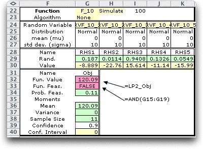
Using the model previously used to evaluate the
mean value solution we simulate this model with the solution
fixed as above. Of course, since the solution is fixed there
is no variability in the objective function. The results indicate
that the solution is feasible for 11% of the simulated RHS vectors.
|
Simple Recourse |
| |
None of the solutions to the No Recourse problem that we have investigated
are very satisfactory. When uncertainty affects the RHS values
of the constraint coefficients there is always a chance that
some constraints will be violated by a fixed solution. Choosing
a solution involves a tradeoff between the risk of infeasibility
and the expected value of the objective function. The table
shows the three solutions considered above in order of decreasing
objective value. Other solutions can be generated by choosing
different satisfaction probabilities for the chance constrained
model.
Solution |
Objective Value |
Feasibility Probability |
| Expected Value RHS |
125.6 |
6% |
| Combined Wait and See |
120.1 |
11% |
| Chance Constrained (90%) |
94.5 |
54% |
The Simple Recourse model explicitly penalizes infeasibility
and maximizes the sum of the linear objective value and the
negative of the expected penalized infeasibility.
Although this model is more satisfactory because it explicitly
penalizes infeasibility, it is much more difficult to solve
than the other models on this page. Obtaining a solution is
probably beyond the algorithms available for Excel. The model
is a special case of the single-stage recourse problem which
is the described on the next page. |
| |
|
|


