 |
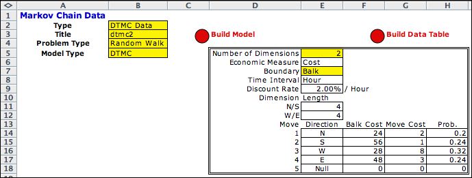
The data form for
the random walk problem is shown below. The structure allows
many alternative assumptions that can easily be accommodated
by the model structure. In the current example we describe
a random walk in two dimensions over a grid with maximum length
of 4 in both directions. The balk costs, move costs and move
probabilities for steps in the four directions are
specified in columns F through G. A Build Table option
is available when the move costs are probabilities depend on
the current state. This
is a Discrete Time Markov Chain (DTMC) model.

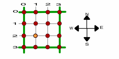
The random walk takes place on the grid illustrated below.
In the example the grid points range from 0 to 3 in each of
two directions. The size of the grid depends on
the corresponding data in column E. We call one direction the
N/S direction and the other the E/W direction. There is a wall
at 0 and another at 3 in both directions.

A walker wanders around on the grid points randomly, and
walls constrain the walker. With the walker at some grid point,
he can move in any of four directions not constrained by a
wall. The example shows the walker as the yellow circle located
at grid point (1, 2). There is a fixed probability of traveling
in any direction and also a cost. When the walker tries to
move in the direction constrained by a wall, a balk cost is
expended, but the walker does not move.
|
Build Model |
| |
Once the data is entered,
click the Build Model button to call the DP Models add-in.
The DP Data add-in calls
the DP Models add-in to construct the model on a new
worksheet. Problem parameters and control buttons are at the
upper-left corner. |
| |
|
| |
The model worksheet holds
descriptions of the states of the model and the events that cause
transitions from one state to another. There are no actions associated
with the DTMC model. The transitions are described by nine transition
blocks. |
States and Events |
| |
The Markov Chain model
requires only the State and Event elements.
The VBA code of the DP Data add-in specifies
the number of state variables and event variables to include
in the model. For this case there are two state variables,
one for each dimension. The state vector is the range
F14:G14. The single event variable identifies the moves with
the indices 1, 2, 3, 4 and 5 representing the directions N,
S, W, E and Null, respectively. With the Null event state
does not change.
Red outlines identify most of the cells that are filled by
the DP Data add-in. Some of the titles that are filled
are not outlined in red to make the figure more readable. .
For example the range F18:G19 holds formulas linking the cell
contents to the corresponding values on the data worksheet. M21
and M22 hold the cost and probability given for the events. |
| |
|
| |
The summary area in
columns O through R indicates whether the State is
feasible and whether the event leads to a feasible transition.
The current state is position (1,2) and the current event is
to move South. The summary indicates that this state is feasible
and that the event leads to a state that is also feasible.
The number in Q20 indicates the transition block defining the
transition. |
Enumeration |
| |
|
The state definition appears
at the left. The state indicates the coordinates of the
current state. Clicking the List Elements button
at the top of the page enumerates all the elements of the
model. The state enumeration is accomplished by changing
the index value in E14 through all integer values from
0 to 15. Sixteen states are discovered and listed on the
model lists worksheet. Details concerning the states are
shown below.

|
|
| |
 |
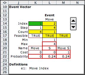
The event definition has only one component
indicating the move. There are five moves, including the
null move. The event probability and cost cells hold formulas
that link to the data worksheet.

|
|
Transitions |
| |
The remainder of
the model describes transitions. With the system in
some state, the occurrence of an event may cause the state
to change. This portion of the model indicates the state/event
combinations that might occur with the associated cost and
probability. Also the model indicates the new state reached
when the event occurs. Starting in row 28 the model identifies
two sets of transitions, those that indicate a balk and those
that result in a move. The order of the transitions is important
since if more than one of the transitions is feasible, the
top one is chosen.
There are four balk transitions with two shown below. Each
transition block is associated with a balk for a certain boundary.
For example, the first transition is only possible when the
current point is at the north boundary. The lower and upper
bounds in cells F36 and F37 are both 0 indicating that this
block is only relevant at the north boundary. The balk occurs
only when the movement is toward the north as indicated by
the lower and upper bounds in L36 and L37. Since the current
state is (1, 2) and the movement is south, these logical requirements
are not met. This is indicated by the FALSE in Q34.
In like manner the conditions for block 2 will be feasible
only when the point is on the south boundary and the movement
is south. For the current state none of the balk transition
blocks are feasible. |
|
| |
The remainder of the
transitions describe moves. There are five of these including
the null move. The first two are below. We focus on transition
block 6 because it is feasible for the current state and event.
Transition block 6 is only relevant when the move is 2, or
south. In that case the new state is shown in row 91. It is
found by adding 1 to the first state variable. The new state
is (2, 2). It's cost, probability and index are in column Q. |
| |
|
| |
The
enumeration process combines all feasible states with all feasible
events. For those combinations that have a feasible transition,
the transition characteristics are listed in the transition list.
The first 28 transitions are below. The balk transitions are
indicated by the high costs. A balk transition does not result
in a state change, but there is a cost. There are 64 transitions
with nonzero probability. |
| |
|
Call Solver |
| |
The DTMC model admits
both the Markov Analysis and DP Solver methods. Here
we have clicked the Transfer to DP
Solver button.
The DP Solver add-in constructs the appropriate
Excel worksheet and the DP Models add-in inserts the
data defined by the model. The probability transition matrix
model for the example is shown below. |
|
| |
The economic transition
matrix is also constructed. The balk costs are on the diagonal
and the move costs are off the diagonal. |
|
| |
The figure below shows
the steady-state solution obtained with the DP
Solver
add-in The green column labeled Last Probabilities shows
the steady-state probabilities. The yellow column labeled State
Value shows the steady-state NPW values. The quantity
in M11 is the expected step value for the solution. |
|
Summary |
| |
This page has demonstrated
the DTMC model for the random walk. The DP
Data add-in constructs a table holding the data.
By clicking the Build Model button
on the data worksheet, the DP Models add-in constructs
the model worksheet and it is filled with the constants and
formulas that implement the model. By clicking the Transfer
to DP Solver button,
the DP Solver add-in creates the solution worksheet
and transfers the information from the list worksheet. All three
add-ins must be installed for all the steps to work.
|
| |
|


