This example comes from a book Dynamic Programming and Markov Processes by Ronald A. Howard, (MIT Press, Cambridge, Massachusetts, 1960). It involves the replacement of capital equipment that ages over time. The model is constructed by the DP Models add-in as described on this page and solved with the DP Solver add-in. The solved model is described on the next page

Creating the Model Form

The data table is at the left. It is placed on the worksheet to the right of the model columns.

Time is measure in three month intervals, called quarters in our model. The time horizon for this model is 10 years, or 40 quarters. Deterioration is indicated by increasing operating expenses over time. The operating expense in column AA is the cost for the next year of operation.

At the beginning of any quarter there is a choice to replace the equipment with a new one, replace it with a reconstructed unit of a given age, or keep the currently owned equipment for one more quarter. The purchase costs of new and reconditioned equipment is given in column Y. The purchase cost of replacement equipment decreases with age.

If the current equipment is replaced, a revenue is realized that is the trade-in value of the equipment. This is in column Z. The trade-in value decrease with age. The trade-in value is less that the purchase cost of the same aged equipment. When the equipment is purchased, the next state is one later than the purchase age. So, when we purchase an equipment of age 0, we next observe it age 1.

The equipment has a survival probability for the next quarter that depends on age as in column AB. A new equipment will certainly survive, while older equipment have decreasing survival probabilities. When the equipment fails it immediately becomes the same as a 10 year old equipment (40 quarters). If it survives the equipment becomes one quarter older.

Equipment that is 40 quarters in age that is not replaced remains at 40 quarters.

Cell AD10 holds the maximum age.

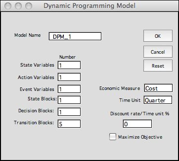
Choosing the Add Model option from the DP Models add-in, opens a dialog box that selects the type of model. Here we have chosen the Stochastic DP option, because we are modeling a Markov Decision Process.

We have decided to model this problem with one state variable, one action variable and one event variable as entered in the appropriate fields. We include one state block and one decision block. These will not be important for this model, but they included in order to retain the option of more blocks later in the problem. We describe the five transition blocks below.

On clicking OK, the entire worksheet is prepared. You should download and open the Replace workbook to follow this discussion. The workbook is saved without control buttons. You can add new buttons with the Start command from the DP Models menu.

The three principal elements are shown below.

The state variable indicates the age of the equipment. It ranges from 1 to 40. The age is observed at the beginning of each quarter. Even if a new equipment is purchased, it will be at age 1 when next observed. The display shows quarter 28. The index in E14 is manipulated by the add-in during the enumeration process. The spinner control in row H can be used to manually adjust the state up or down during model debugging. There are 40 possible states.

The action variable indicates the decision at the beginning of each quarter. For this discussion use x to indicate the action. When x = 1, shown here, the equipment is kept for one more quarter. Other values of x means to trade in the current equipment and purchase a replacement of age x - 2. Thus x = 2 means to purchase a new equipment. When x = 41, the action is to purchase an equipment of age 39. There are 41 possible actions and each is available in any state.

Cell K21 contains a formula that describes the cost of an action. The formula includes an Excel IF function that depends on both the state (s) and the action (x). The cost is for the next period and looks something like this:

=IF(x=1, OE(s + 1), -(TD(s + 1))+P(x - 1)+OE(x - 1))

The indexing may seem odd, but it is due to the action being 2 greater than the purchase age and table index being one greater than the age. For the keep action, the cost of keeping an equipment of age 28 for one more quarter is 141.

There are two events represented a binary variable with 0 indicating failure and 1 indicating success. Costs and probabilities depend on both state, action and event and computed in the transition blocks. The entries in rows 21 and 22 are the default values.

To the right of the figure starting in columns S is the summary for this state/action/event combination. It indicates that the feasibility conditions for state, decision and transition are all satisfied for this combination. We must look into the remainder of the worksheet to see what this means.

State and Decision Blocks

The model has one state subset block and one decision block. They perform no function for this example. The default values supplied here do not limit or change the objective terms already defined by the state and action variable definitions.

Transition Block 1

The first transition block is feasible when the age of the equipment is less that 40 (the max age), the action is to keep the equipment and the event is a success. These conditions are implemented by the bounds in rows 61 and 62. If all this combination is true, the transition simply increases the age of the equipment. The number 1 is placed in cell F64 to accomplish the transition. The new state is indicated in row 66 as age 29. It's index in the state table is also 29. Cell H66 is TRUE when the next state is in the state table.

The probability of this event is placed cell U61. That cell contains a formula that points to the probability column of the data table for the row determined by the current age. You will find the number 0.85 in the table for age 28. We call a number from this table p(s). The entry in cell U61 is p(28)

Transition Blocks - Keep

The figure below shows both block 1 and block 2. In this case we are viewing the effect of the event of a failure. The event variable is 0. Because the bounds in the event section of block 1 are both 1, the first transition block does not describe the current combination. This is indicated by the expression FALSE in U60.

Block 2 was designed for this kind of combination as the bounds on the event are both 0. Cell F74 holds the expression: 40 - s. This evaluates to 12 for the current state and the result is a transition to state 40. This is the result of the failure event.

The expression for the probability in U71 is: 1 - p(28). This is the probability of failure for age 28.

Transition Blocks - Buy

Transition blocks 3 and 4 describe the transitions for the Buy action. For these blocks the action variable ranges from 2 to 41. All ages are allowed by the state range. For illustration we use the action 6, buy an equipment of age 4. Block 3 describes the event of success for the next quarter, and block 4 describes the event of failure. Note that the transition in block 3 results in a new state representing age 5. A failure, block 4, results in a transition to age 40.

The transactions for the process are assumed to occur at the beginning of the quarter, so the probabilities of success or failure depend on the action, not the state. The formula for the probability in block 3 is p(x-1) and the probability of failure in block 4 is 1-p(x-1).

Transition Block - Age 40

The Complete DP Model

Before constructing the transition blocks it is important to click the List States button at the top of the page. A transition box will not be effective unless the transition leads to a feasible state. A state is judged to be feasible when it is in the State List. To review the lists implied by the model click the List Elements button. The add-in enumerates all states and actions to construct the state, action and event lists. Then the add-in enumerates all feasible states and actions to find the decision list. In this case all actions are feasible in all states, so we have 1640 rows of the decision list. There is two transitions in each state. Deleting the transitions with zero probability there are 3239 transitions.

The example is interesting because the state space is small with only 40 states, while the decision space is large with over 1600 decisions.

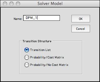
Clicking the Transfer to DP Solver button creates the lists. builds a DP Solver form, and transfers the model lists to the DP Solver form. We choose the Transition List option, but the other options are also available because of the small number of states.

The DP Solver model for this problem is on the next page.