|
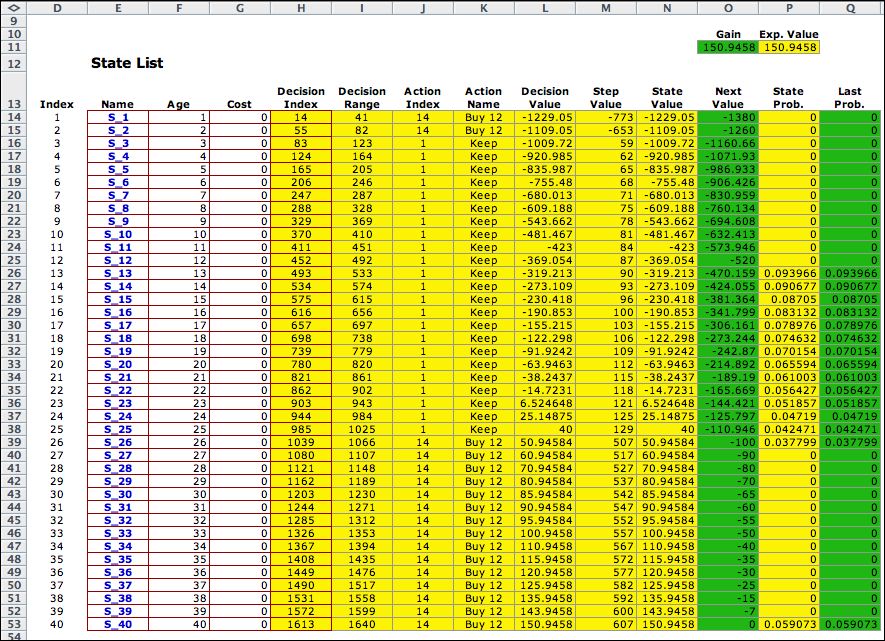
The state list for
the replacement problem is shown with the initial assumptions
regarding the Next Value and Last Probabilities.
The decision and transition lists are to
the right of this display. |
|
| |
|
Since there are a relatively small number
of states for this problem, we choose the Policy Iteration method.
This methods solves a linear set of equations at each step
to find the values associated with the states for a fixed
set of decisions. Using these values, a one-period optimization
is performed to find better actions. If no improvement
results, the process stops. Otherwise the values are found
for the new solution. This process will terminate in a
finite number of steps with the optimum policy. |
|
| |
The optimum solution
is shown below. The discount rate for this model is zero. With
a zero discount rate the objective can no longer be the net
present worth. When the average cost be step is positive, the
NPW is unbounded and the with an infinite time horizon. The
method proposed in the Howard book minimizes the average cost
per period, per quarter in the example at hand. A different
set of equations is solved by the Policy method. The equations
determine the relative values of the different states when
the value of one of the states is fixed at zero. The average
cost per period is also determined by the equations. It is
placed in the cell labeled Gain in the figure below.
Notice that the Gain is the same as the Expected
Value. The Expected value is computed by multiplying the
state probabilities times the Step Value. It is the
long run expected value per period of operating the system.
For a specified policy, the system is a Markov chain with
a single set of recurrent states. For the example, the recurrent
states are those with nonzero probabilities in column P. The
rest of the states are transient. The values in column O come
from the solution of the equations. Since all the states have
negative values in row O, it is profitable to start in any
state than state 40. |

|
|
Notice the optimum policy is to
purchase a 4 year old equipment (12 quarters) and hold it until
the age is 26 quarters. Then at the 27th quarter trade the equipment
of one that 12 quarters old. State 40 is part of the recurrent
states because there is almost a 6% chance that the equipment
will fail. When that happens, replace the failed machine with
one that is 12 quarters old. States 1 through 11 and also states
27 through 39 are transient. The system can start in any of these
states, but the optimum policy is to immediately switch to the
12 quarter old equipment. |
Sequence of Solutions |
| |
It is interesting to observe the
sequence of solutions obtained by the Policy iterations.
The first four steps are shown in the figure below, and the last
three steps immediately follow. The policy migrates from the
initial solution, through a series of intermediate solutions,
and finally reaches the optimum where no improvement is possible.
This process minimizes the expected value of one period of operation.
This quantity is computed for each iteration in row 7. As expected
the values decrease monotonically to the optimum value of 150.946. |
|
| |
The sequence shown is exactly that
obtained in Howard's book. |
Summary |
| |
The example is interesting in that involves
a fairly large number of possible decisions. The computations
required are well within the capabilities of Excel.
|
| |
|


