Revenue management is one of the successful applications of operations research. It is used throughout the transportation industry and could be valuable whenever a business has a fixed capacity resource that is used on a regular schedule. Examples are airline flights, hotel accommodations, batch processing machines and many others. All these examples require a major fixed cost for providing a service. The cost is independent of the number of customers who pay to use the service. To maximize profit, the business wants as many customers as possible who individually pay a high price for the service. In most cases there is tradeoff between these goals. The maximum number of customers can only be obtained with a low unit price, and the highest unit price results in the fewest customers. Since the cost is fixed, the goal is to find the combination of pricing and customer demand to maximize total revenue. This problem is addressed through revenue management. The example on this page is one of the simplest of the revenue management problems.

An example is an airplane used in a commercial setting.

The commodity for sale is an airplane seat. Although every seat performs the same function of carrying a customer from one city to the other, various benefits can be made available to allow some seats to be priced higher than others. Benefits include early check-in, free drinks, pillows or blankets. Lower priced seats do not enjoy these perks and are more restricted. Restrictions include the inability to change or cancel the reservation or the requirement to stay at the destination city over Saturday night. Some tickets might be offered at lower prices just before the flight. Selling a ticket for a seat that would otherwise be empty always increases the total revenue.

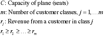
In some manner, the market for the product must be segmented into several classes: 1, 2, … m. The classes have different prices with the price decreasing with increasing class index.

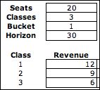The data at the left is used as an example. The capacity of the plane is 20 and there are three price classes. Time is divided into buckets, here defined to be one day long. Tickets are available 30 days before the flight leaves (the Horizon).

Reservations

The flight leaves at a scheduled clock time. We divide the time before the plane leaves into equal intervals called buckets. The buckets are numbered to indicate the number of buckets before the plane leaves. The plane leaves at time 0. One day before departure is time 1, and so on. N is the number of time buckets between when the airline begins to sell tickets and when the plane leaves.

Customers make reservations though the internet. To control the number of customers that will be accepted from each class, each time bucket is assigned a class number that indicates the maximum class index that is acceptable.

For this problem we assume that only one reservation is booked during a time bucket. Customers in the different classes arrive independently at random times described by a Poisson process. The action is to specify the value of x for each state in each time bucket. We assume that the first acceptable customer that arrives during a bucket is booked. Customers arriving later than the first in a bucket are lost. This may seem to be an unrealistic assumption, but the model can be made more accurate with smaller duration buckets.

The chart below shows one solution for the problem. The horizontal axis is the number of days until the flight departure. The vertical axis is the number of seats that are full. The colored cells indicate the policy for each combination. For green cells, reservations are accepted for all three classes. In yellow cells, reservations are allowed for classes 1 and 2. Only class 1 is accepted in the red cells.

A solution like the one shown is reasonable. When there is only day to go, empty seats should be sold for any price, since a seat not sold provides zero revenue. At earlier times when only a few seats are left, it is better to restrict reservations to make sure there is opportunity for higher paying customers to buy seats. Early in the reservation process, it is better not to sell the cheaper tickets so that space will be available if more expensive tickets are requested later. No reservations are accepted when the state reaches the capacity of the plane.

In the MDP model the state variable is the number of booked seats, and the stage variable is the time bucket index. The chart shows the optimum actions. For bucket 1 the decision is 3 for all states less than 20, the capacity of the plane. For bucket 2, the decision is to accept reservations of all types unless the state is 19, one less than the capacity. In state 19 we book only classes 1 or 2. In bucket 30, reservations begin with no seats booked, no reservations are accepted at price 3.

The time between arrivals for each class is assumed to be exponentially distributed. Different classes have different arrival rates. The exponential assumption allows computation of the probability that no acceptable arrival occurs during the time bucket and the probability of booking a customer from each acceptable class. For this model we assume that arrival rates are independent of time, so the parameters are not indexed by the bucket number. This means that the model is homogeneous in time.

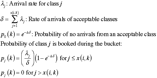
The decision problem is to assign a class index to each state and each time bucket. No reservations are accepted for classes with indices at above the maximum. The goal is to maximize the expected total revenue over the time horizon.

Model

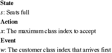
We model this problem as a Markov decision process (MDP). The number of seats taken is the state variable. The stage variable is the bucket index. Since the model for each stage is the same, the stage variable does not appear in the model formulation. You will see that the effect of time is considered by the computational process of solving the model. The action is the selection of the maximum class index to admit. The event is the index of the class of the arriving customer. The figure shows the state, action and event variables defined on the DP model worksheet.

The example shows the model with 10 seats full, the action is to accept reservations of class 1 or 2, and the event indicates that a customer of class 1 has arrived during the interval. The ticket is booked. The event element holds formulas that describe the revenue and probability associated with the event. These formulas link to a data table constructed to the right of the model and illustrated below. Changing this data automatically changes the related cells of the model.

The event of no arrival is modeled implicitly. When the DP Models add-in creates the model, it automatically creates a null event that holds all unspecified probability for a given state/action combination. This null event represents the situation when no acceptable class arrives during a time bucket.

States

Transitions

Lists

When the add-in is called to generate the solver model, five lists are created as shown below.

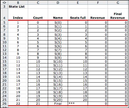	The state list shows all possible states for the system. A Final state is necessary for the transition from state 20 to the exit.
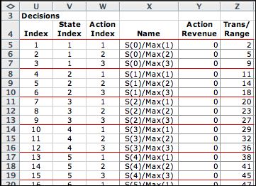
	The three actions are to set the maximum acceptance index to 1, 2 or 3.
	The event list shows the classes that might be booked during the time bucket.
.	There are 62 state/action combinations, or decisions, that are feasible for the model. State 20 allows only the Null action.
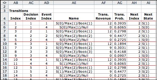
.	There are 182 transitions for this model. The transitions carry the revenue and probability information.

Optimization

Clicking the Transfer to DP Solver creates the five lists and transfers them to the solver model worksheet. The solution is on the next page.