Computation - Operations Research Models and Methods

Computation

Dynamic Programming

DP Examples

Revenue Model

Revenue Solution

Excel Page
Download

	Dynamic Programming Examples
	- Revenue Management Solution

Clicking the Transfer to DP Solver button on the model worksheet creates the solver worksheet and transfers the five lists to the data portion of the worksheet. The upper-left corner of the worksheet is shown below. The full worksheet can be seen by downloading the revenue.xls workbook. The information in column B shows the summary with the initial conditions.

The state list for the problem shows the Value solution for the first step. This is the last day before the plane leaves. It is optimum to open registration to all classes regardless of the number of seats full. The state values are all the same. This is the expected revenue for the last day only.

Clicking the Solve button presents the Solver Dialog. For a finite horizon problem, set the number of iterations to the time horizon. Each iteration describes the passage of one day. We initialize the state values to 0 because no additional revenue can be earned after the plane leaves. The probabilities do not play a role for finite time horizon problems.

Select the All button in the Show Iterations panel. The intermediate results are important for finite horizon problems.

Clicking the OK button on the Solve dialog presents a dialog for selecting the intermediate information to display. For this problem we choose to show only the actions. The set of actions for the 30 days describe the optimum policy.

After 30 steps, the state display shows the optimum policy for 30 days before the flight leaves. This is the first day for accepting reservations for the flight. Assuming that one begins with zero seats full, only the first row of the table is important. The optimum policy is to open reservations for classes 1 and 2.

The value in the first row, $202.38, is the expected revenue for the flight. This is higher than the operating cost of $180, so the optimum policy results in a positive net profit.

The remaining lines show the optimum policies and expected revenues for more seats full. This is equivalent to evaluating the optimum policies for smaller planes.

Optimum Policy for All Days

The States worksheet displays the optimum policy for all days. After adding conditional formatting to the cells, the optimum policy is clearly displayed by the colors on the chart below. Although the model does not change over time, the policy changes quite markedly to reflect the finite horizon of the problem.

Time Variable Arrival Rates

In a more realistic representation, the model will change over time when different classes of customers have time-variable arrival rates. Model Rev1on the example worksheet describes this kind of model. Because the solver worksheet shows the entire model explicitly, modifications of the model can be implemented using functions of the step number. For this case we use the tables below to describe the variable arrival rates.

time variable data

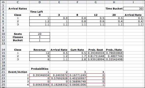
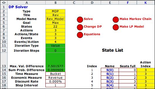
The table at the top shows the arrival rates by class during five time intervals. The first column (Col. D, labeled 0) shows the arrival rate for buckets 1 through 2. The second column shows the arrival rates for buckets 3 through 7, and so on. The current day is in cell I2. This number is transferred from B12 on the solver worksheet. The current arrival rates are in cells I5 through I7. They are obtained from using an Excel Lookup function. The arrival rate is transferred to the tables below. Ultimately, the bottom table computes the transition probabilities for each event under each actions. Action 4 is the null action and event 4 is the null event.

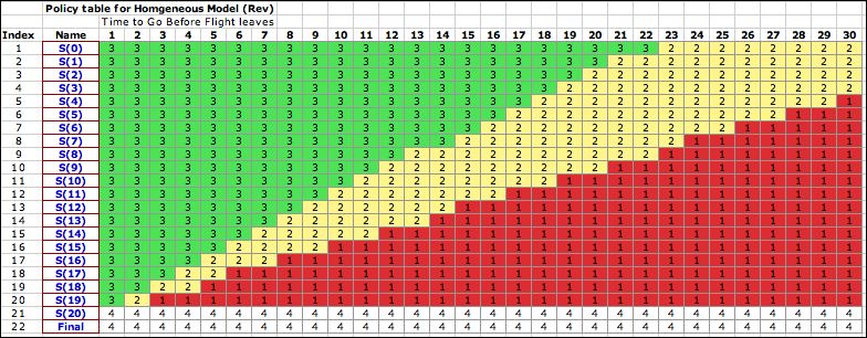
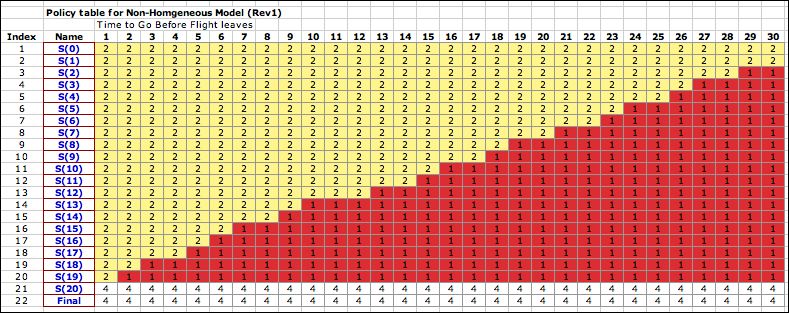
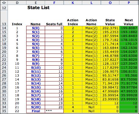
The probabilities are transferred to the transition probability column on the solver worksheet using the INDEX function. Now as the iterations progress, the transition probabilities depend on the bucket number. The policy now reflects the new model. The figure below shows the optimum policy over the time horizon. It is never optimal to offer the class 3 ticket.

Summary

Finite time horizon problems can be solved using the DP Solver add-in by performing Value iterations for a fixed number of steps. The optimum policy over time is obtained by recording the optimum action at each step.