[The following solution was derived from the original Harvard Business Review Case Studies. There are other possible solutions, but the following one yields stable long run minimum costs. See also one of these alternate solutions just developed, at the end of this one.]

The solution to the P&G soap packaging line simulation is based on answers to the following four questions:

1. At what level should the original production level be set?
2. When should a change in production level be made?
3. How much should the change be?
4. How do we plan for the plant shutdown for vacation?

We will start with the third question. Since the cost of changing production is relatively high, we will make the largest possible change possible, +/- 10 units, so as to spread this cost over as many units as possible and cut down on the number of changes.

We will now consider the second question – when to change the level of production. The key variable is the ENDING INVENTORY. We are dealing with three types of variables – controllable (PRODUCTION LEVEL), uncontrollable (DEMAND) and the dependent variable (ENDING INVENTORY). The following relationship shows the connection.

Beginning Inventory + Production – Demand = Ending Inventory.

The Ending Inventory of one period is the Beginning Inventory of the next period.

Since the average weekly demand is 100, we would like the Ending Inventory to be around 100. This would be viable if the demand was steady. However, the standard deviation of demand is 30 units. This means the demand from week to week could vary between 70 and 130 about 2/3rds of the time, between 40 and 160, 95% of the time and between 10 and 190, 99.8 % of the time.  Such variation is difficult to handle. A measure of variation used is the ‘Coefficient of Variation’ – defined as the ratio of the standard deviation to the mean.

COV = STD DEV / MEAN

If this measure is less than 5%, then the variation is can be considered ‘noise. If it the between 5 and 15 %, this is considered somewhat variable. About 15%, the variation is considered WILD. Our value is 30%! So we have a problem. This coupled with the two week delay in changes going into effect can cause severe problems, mainly large shortages. Therefore, we need to establish ‘control limits’ in the value of Ending Inventory. These limits are similar to those used in Quality Assurance Control Charts.

If the Ending Inventory is around 100, we will want our production to be 100. As Ending Inventory exceeds 100, we will want to have less production so as to ‘boil off’ the excess inventory and get back to 100 and reduce our inventory holding cost.

If the Ending Inventory is less than 100, we will want to increase production to avoid stock-outs and the high penalty costs.

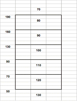
Below is a possible set of limits based on the original P&G case study. The numbers on the left describe the ending inventory and the numbers in the middle give the desired production level for ranges of the ending inventory.

This chart also answers the first question. Since the initial inventory available is 270 units, this is way above the upper most limit and we set the initial production level at 70 units.

As the demand for each week is known, we can determine the ending inventory. (Actually, the simulation does it for you.) When the ending inventory falls below 190, the table indicates that we need to increase production – by 10 units.

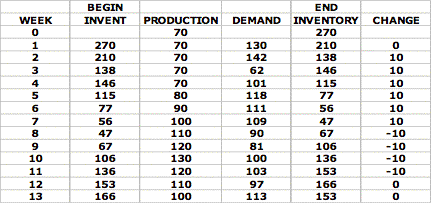
To illustrate the use of this chart, we have summarized the first dozen weeks of an actual simulation below

Since the beginning inventory is 270, we set the initial production level at 70. At the end of the first week with a demand of 130, the ending inventory is still above 190 so we make no change. In week 2 the demand is 142 and the ending inventory is reduced to 132. By the chart we want the production level to be 90, so we increase production by 10. Note, this will raise it only to 80 so we may have to raise it again in the next week. (To keep track of where we are, we can simply Put a token on the chart at production level 80.) (A coin will do – a penny or dime for current production.)

The next week demand is low – only 62 and the ending inventory is still in the 130-160 range for a production level of 90. But we are still at 80, so we raise it again. In the next four weeks, the demand is relatively high and the ending inventory falls to a low of 47. So each week we raise it by 10 until we are at the 130 level. This ‘catch-up’ takes effect and ending inventory starts to rise and as it does and enters a new range, we start to lower production with -10 changes. We would continue using this strategy throughout the simulation.

At this point, it appears that we have made an excessive number of production changes. The alternative is to make fewer changes and the result could be disastrous. With the two week delay in implementing the production level change and with the greatly varying demand, the ending inventory could sink to extremely low levels and recovery could take weeks. It is better to exercise more precise control.

The other tendency is to relax when changes are made. For example, if the ending inventory were to barely move into a new range, say from 155 to 162, the urge may be to delay making a change. Again this could be bad. The idea is to make these changes almost automatic, i.e. program a computer to do them.

The final question is, ‘How to prepare for the plant shutdown in weeks 26 and 27 when no production is possible. We know that during this two week period, the average total demand should be 200. While it is possible that we could have two weeks of extremely high or extremely low demand, this is not likely. (The standard deviation for this two period of demand is 42.42. So 2/3rds of the time the two demand would range from 158 to 242 and 95% of the time from 115 to 285.)

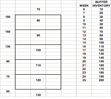
What we need to do is build up a ‘buffer’ inventory of 200 units to cover this period. The way we do this is to ‘set aside’ 10 units a week for 20 weeks. We do this by ‘subtracting’ this increasing buffer from the actual inventory to arrive at an ‘effective’ inventory and base our decision of production change on this amount. We start this in week 6 and continue to week 25.

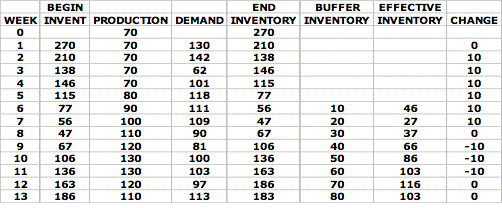
To illustrate the use of this table, we again show a portion extracted from the simulation, below.

In this simulation, we have generated the same random sequence for demand as before, so that we can compare with our previous analysis. The production changes are the same thru weeks 1 – 5.

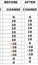
In week 6,  we begin to use the ‘Effective Inventory.’ However this does not result in any different from before. It is in the 8^th week that a difference occurs. The effect of the buffer inventory is to show the effective inventory still at a low level. Therefore, we delay the change to decrease production. A comparison of the two is shown below.    

The overall impact of using this strategy, is to keep product levels high to build up the buffer inventory to prepare for the plant shutdown. This has two effects. First inventory costs will be slightly higher. Second, the probability of a stock-out will be lower especially as we get closer to the plant shut-down when the buffer becomes large. So the possible stock-out cost is reduced.

Employing this solution method does not guarantee a shortage will not occur. The total cost will vary from simulation run to run. With this method, the average total inventory cost is around $135,000. The lowest seen is $65,000 and values near $250,000 are not unusual. Without using a good strategy, some users have had costs approaching one million.

This is not the only effective strategy. We have seen one about as good, but it has been lost for decades. Perhaps you will rediscover it or one even better.

         William G. Lesso

         October 20, 2006

The following solution was developed by
Mr. Hiroki Abe
Offshore Iwaki Petroleum  Co Ltd.

 During a recent workshop (Dec, 2006), Mr. Abe was asked to play the PNG games several times. After the first play, he was asked to develop a strategy, write it down and play the game again using his strategy. This strategy, given below, is quite simple and gave consistently good results. You might want to try it.

•   Set initial production at 100.
•   All production changes are to be only +/- 5.
•   Let Ending Inventory build up to the300-350 range by increasing production.
•   Keep it in this range by +/- production changes until after the plant shutdown.
•   After the plant shutdown, keep Ending Inventory in the 100-159 range until the end of the game.

I do not recall if Mr. Abe specified and upper or lower limits to production levels but I believe the changes in production should keep overall production between 70 and 130 or perhaps between 50 and 150 if one is adventurous