The mathematical model below provides notation for aspects of the portfolio optimization problem. The portfolio is defined by the proportion of the investment in each security. The proportions must sum to 1 indicating that the entire portfolio consists of the candidate securities. Whether the returns for the securities are independent or not, the expected return is a linear function of the mix components.

Independent

When the security returns are independent, the value of the return for one security does not provide any information about the values of the others. Although this is probably not a good assumption for investment securities, consideration of the independent case provides justification for the policy of a diversified portfolio.

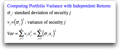
The variance of the portfolio is sum of the variance contributions of the individual securities. An individual contributes the variance of the security multiplied by the square of the proportion. Since proportions are all less than 1, low variance solutions are comprised of a mix of all available securities. A randomly generated example provides an illustration.

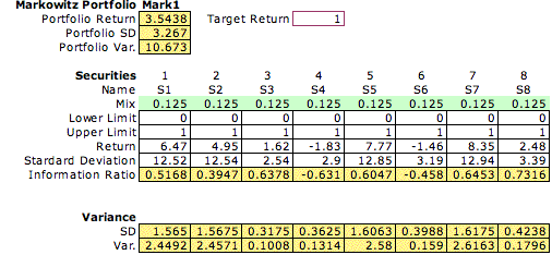
Considering the solutions on the efficient frontier, we see that the solution with the smallest standard deviation has representatives from all the securities, even those with a negative return such as S4 and S6. As more and more return is demanded from the portfolio, these securities drop from the mix. The highest return portfolio has a single security, S7, and the greatest standard deviation.

Correlation

Computation of the portfolio variance becomes more complicated when the returns are correlated.

We use the last expression for computing variance because the correlation matrix is often available from published sources. An example involving correlation is below.

The spreadsheet model computes the variance in two parts shown in the bottom row and the two right most columns. The variance is the matrix product of the bottom row and the right most column.

The frontier analysis for the example again shows the benefits of diversity.

Math Programming Model

The optimum mix is found with a nonlinear mathematical programming model with two constraints. The first constraint requires that the mix proportions sum to 1. The second constraint requires that the mix provide at least an expected return P. We call this the target return. The objective function is a quadratic function of the mix proportions.

The implementation of this model in Excel is illustrated below. The model is created by the Math Programming add-in and solved with the Excel Solver. During the solution process, the variables of the math programming model in row 8 are linked to the mix variables in row 27. The entry in cell H13 is linked to the portfolio variance computed in cell I23. The coefficients of the return constraint come from the values entered in row 30, and the lower and upper bounds in rows 9 and 10 come from the lower and upper limits for the proportions entered in rows 28 and 29.

The Solver manipulates the row 8 values in the search for a minimum variance solution that yields the target return in L22, in this case 10. The optimum solution is reported in row 8 and copied to row 27. For simplicity, the math programming model is hidden when the model is first constructed. The model can be viewed by clicking in the cell in the upper left hand corner and choosing to Unhide the rows.

Although the math programming model is easy to state, it is not necessary easy to solve. With correlation, the portfolio variance is a difficult computation when there are many variables. The number of terms in the expression is proportional to the square of the number of variables. Since the Excel solver evaluates this nonlinear expression many times, the solution process will be slow when the number of variables exceeds 20 or 30. Although the Solver may not be reliable when there are a number of variables.

Since the objective function is a convex quadratic function, the solution could have been approached by quadratic programming. We have chosen this simpler nonlinear programming model for the add-in.

Commercial solvers are probably faster and more reliable than the free Solver that comes with Excel.

Additional Variables and Constraints

The nonlinear programming model can be expanded to handle extra variables and constraints that financial planners might impose. Simple lower and upper bounds on the individual mix proportions are already accommodated by the model. Restrictions on collections of securities can be added by specifying additional constraints in the dialog defining a model. Those familiar with math programming can easily add linear constraints to the model and the difficulty of finding solutions is be greatly increased.

It is also possible to add 0-1 variables that model the selection of individual securities. These might be used to limit the total number of securities included in the mix. Adding integer variables is possible for a convex programming problem, but finding solutions will be much more difficult for the Solver algorithms.