|
|
 |
Materials
Requirement Planning |
 |
-MRP
Formulas |
|
|
The
yellow areas of the MRP worksheets contain Excel formulas.
These formulas are constructed by the MRP add-in. Although
the formulas can be viewed directly on the worksheet through
the Formula toolbar, it is hard to interpret them
in mathematical form. This page provides a mathematical
basis to the computations. |
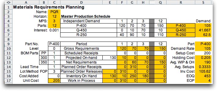
The Gross Requirements |
| |
The computations
for a given part are driven by the Gross Requirements for
the part. When a part is represented in the master production
schedule, the gross requirements for the part are the values
entered as the independent demand for that part. This is illustrated
in the figure below for P-400. The Link Parts command
places formulas in the gross requirements row of P-400, row 10
in the figure, that reference the cells giving the independent
demands for P-400. For example the cells in row 10 all have the
formula:
=PQR_MPS_Prod_1
The reference is to the independent demand in
row 5. |
|
| |
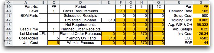
Some parts are mentioned in the
Bills of Material (BOM) of other parts. In this case the formulas
that define the gross requirements are more complicated because
they depend on the BOM entries of one or more parts. A given
part may have independent demand and also be in the BOM's
of one or more other parts. Part PP is included as the BOM
of P-400. The formula in the yellow cells of row 40 is
=INDEX(PQR_BOM1,1,2)*PQR_Part1_Rel
Before the multiplication symbol, *, the formula
references the BOM of P-400. After the multiplication symbol,
the formula references the planned order releases of P-400.
The demand for a component depends on the planned order releases
of the part. In general the formula may references several
parts and be quite complex. |
|
Formulas for the Parts |
| |
Given
the gross requirements, scheduled receipts, and the initial
on hand inventory, all the other entries on a part form are
computed with mathematical formulas. We adopt the following
notation for the part quantities. For this section we are assuming
a fixed lot size.

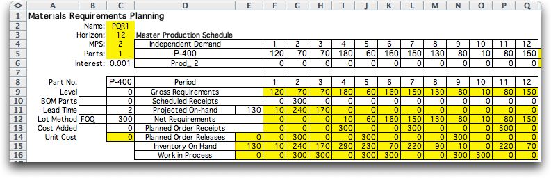
To illustrate we use the P-400 part with
the fixed order quantity (FOQ) lot method. Whenever the inventory
would otherwise become negative, this policy requires the receipt
of a fixed lot size. In the example, the lot size is fixed
at 300. The initial on hand inventory is 130. A delivery of
a lot of 300 is scheduled for time 2. The order for this lot
was placed prior to the beginning of this time horizon. Note
that the lead time is 2. The lot size, on hand inventory, scheduled
receipts, and lead time are all entered on white cells indicating
that these entries are data. |
|
| |
Indices on the quantities
range from 1 to T, the time horizon. The time horizon
is 12 for the example. In some cases the index of 0 indicates
the initial value. |
|
|
Rows
of the Part Form |
| |
Quantity |
Explanation |
 d d( t) |
Gross Requirements |
For this discussion of the part
formulas, the gross requirements are given. For the example,
the gross requirements are specified as data in row 5. |
e(t) |
Scheduled Receipts |
The numbers in this row are quantities
not scheduled on this form. The numbers in this row are
data. |
h(t) |
Projected on-Hand |
The initial value is a given,
but the remaining values are computed with the formula:
|
n(t) |
Net Requirements |
The requirements that cannot
be met with projected on-hand or scheduled
receipts are the net requirements. These must be satisfied
from production during the time horizon.
|
x(t) |
Planned Order Receipts |
These are computed based on
the net requirements and the lot sizing method. The
example uses a fixed order quantity of 300. If
the inventory at time t - 1, plus the scheduled
receipts at time t, less the demand at time
t, is negative, an order is planned to be
received at time t. The order is the specified
lot size unless the lot size cannot meet the demand.
If the fixed lot size cannot satisfy the net requirements,
the order is the net requirements less amount on hand.
This order size assures that the inventory will never
go below zero.
|
y(t) |
Planned Order Releases |
If an order is to be received
at some time, the order must be placed L periods
earlier. This is accomplished by setting the planned
order release equal to the planned order receipt L
periods later. The top condition requires that
the time of receipt must fall within
the time horizon.
|
z(t) |
Inventory on Hand |
The inventory on-hand is the
previous inventory, plus planned receipts, plus scheduled
receipts, minus demand.
|
w(t) |
Work in Process |
This work-in-process is
the number of units released to production,
but not yet received.

|
|
| |
| The
column at the right of each part data computes averages
over the time horizon. |
| Quantity |
Explanation |
| Demand Rate |
The average demand per period over
the time horizon. |
| Setup Cost |
The cost for a production run for
a manufactured part or an order for a purchased part. This
is data. |
| Holding Cost |
This is the cost of holding one unit
for one period. It is computed by multiplying the Unit
Cost by the Interest Rate. |
| Average WIP and OH |
This is the average over the time
horizon of the number of units in production and in inventory. |
| Average Setup |
This the average number of setups
per period. |
| Inventory Cost |
This is a measure of effectiveness
for the scheduling policy. It adds the cost of holding
WIP and inventory and the cost of setups. An optimum policy
would minimize this value. |
| EOQ |
Economic Order Quantity. This is
the optimum lot size based on the averages over the time
horizon. It is computed with the standard EOQ formulas. |
| EOP |
Economic Order Period. This is the
optimum period between orders assuming demand is continuous
over the time horizon and the EOQ is used. |
|
| |
The
MRP worksheet uses only native Excel formulas. The add-in constructs
the worksheet and inserts all the required formulas. |
| |
|
|