| |
The economic analysis for the system is shown below. Data in
white fields are provided by the user, while numbers in yellow
fields are Excel formulas. Assuming sales at their maximum values,
the system generates a net income of $7350. Goldratt would call
this the throughput of the system. It is the revenue
from sales less the cost of raw materials. The operating expense
of $4500 should be deducted from this figure to obtain the profit
for the system.
The unit-raw material costs for each product are computed and
shown in column J. Column K holds the unit-operating profit
for the products. Goldratt would call these numbers the unit-throughput
values for the products.
|
|
| |
This solution may or may not be feasible with respect to the
resources available for production. The resources are represented
by the times available for the machines which are shown in the
table below. The add-in creates the list of machines (resources)
used from the four products. For each machine, data specifies
the number, time available, percent available and maximum utilization.
The results of columns K through M are computed from this data.
Column N shows the amount of each resource used for the sales
quantities entered in the table above. Column O shows that only
machine B exceeds 100% utilization, so this machine must be
the bottleneck. We also note that machine R is a potential source
of problems since its utilization is 95%.
|
|
|
| |
We could stop at this point with
the bottleneck identified, but we continue to illustrate the
next step of analysis.
The foregoing analysis has neglected a number of features associated
with the situation. An important factor for all real systems
is statistical variability. Although the data presents operating
times and setup times as single numbers, these times may vary
from unit to unit and from lot to lot. Machine time can also
be lost due to failures. Although machine B is barely a bottleneck
with its utilization exceeding capacity by only 1%, statistical
variability assures that the machine can probably not be operated
at full capacity. One way to plan for this is to set the maximum
utilization in column K to some number less than 100%. In the
table below, we set the maximum utilization to 90%. Now the
resources used by machines B and R exceed the resource available
indicating that there may be two bottlenecks. |
|
|
| |
With bottlenecks in the system, we
cannot manufacture the entire weekly requirements. Rather, we
must select a product mix that maximizes total throughput (net
income on this worksheet). The add-in provides access to a linear
programming model to find the optimum product mix. To create an
LP model click the Build LP/IP model button on the worksheet.
|
 |
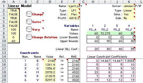
The LP model describing the
product mix problem is shown below. All parameters of
the model are determined automatically from the process
and economic data. The model has already been solved in
the figure below.

Review of the solution shows that the full
production of finished good C is not met by the optimum
solution. Column D shows the amounts of the resources
used by the solution. Clearly machine B is a bottleneck
since all of its capacity is used. Machine R is not a
bottleneck because the solution does not use all of its
available capacity.
|
|
| |
Returning to the Project
worksheet we find that the sales per week have been translated
from the LP solution. There is a reduction in net income from
the unconstrained case. The resource utilizations are all less
than 90% as required for this solution. As expected the resource
utilization for machine B is exactly at 90% while all the others
are less.
|
|
| |
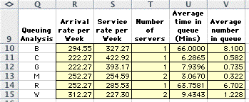
The Project worksheet
provides a queuing analysis for the machines. The queuing model
assumes that units are processed independently with Poisson
arrival and service processes.

Although one might argue about the validity of
the queuing analysis assumptions, these results do show the
affects of statistical variability. The bottleneck machine has
the greatest queuing delay, while the near bottleneck, machine
R, also shows considerable delay. The delays at the less utilized
machines are much smaller.
|


