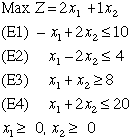
This problem considers the linear programming model shown below.

Solving this problem we obtain the solution:

Sensitivity analysis obtained from the computer program is
shown below.
Dual Solution
|
Row
|
Constraint
|
Value
|
|
1
|
E1
|
0
|
|
2
|
E2
|
0.75
|
|
3
|
E3
|
0
|
|
4
|
E4
|
1.25
|
Simple Ranging for Objective Function Coefficients
|
Variable
|
Objective Coefficient
|
Lower Range
|
Upper Range
|
|
x1
|
2
|
5
|
---
|
|
x2
|
1
|
-4
|
4
|
Simple Ranging for Right Sides of Constraints
|
Constraint
|
Right Side
|
Lower Range
|
Upper Range
|
|
E1
|
10
|
-4
|
---
|
|
E2
|
4
|
-10
|
20
|
|
E3
|
8
|
---
|
16
|
|
E4
|
20
|
9.33
|
---
|
Use this information to answer the following questions.
a. Explain what the entries in rows 1 and 2 indicate in the
dual solution table.
b. Explain the upper and lower ranges given for the objective
function coefficient of x2. What
remains constant as the coefficient is changed within the range?
Hold all other problem parameters constant.
c. Explain the lower and upper limit given for the range on
the right side of constraint E2. What remains constant as the
right side is changed within the range? Hold all other problem
parameters constant.
|

