A product is produced at two manufacturing plants and shipped
to 3 sales outlets. The unit revenues and the maximum sales at
the outlets are shown in the table below.
|
Sales Outlets
|
A
|
B
|
C
|
|
Revenue per unit
|
$20
|
$30
|
$25
|
|
Maximum sales
|
10 units
|
20
|
10
|
The data below shows the unit costs and maximum productions
at the plants.
|
Manufacturing Plants
|
I
|
II
|
|
Cost per unit
|
$6
|
$8
|
|
Maximum production
|
30 units
|
30
|
The data below shows the shipping costs per unit between plants
and sales outlets.
|
Sales Outlet
|
A
|
B
|
C
|
|
Plant I
|
$4
|
$8
|
$6
|
|
Plant II
|
$6
|
$3
|
$10
|
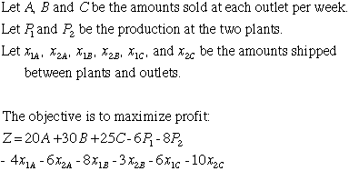
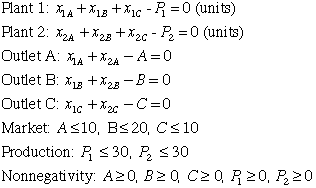
The linear programming model for this situation is shown below.

subject to:

In each of the following three problems we modify the situation
in some way. Show the change in the model. When solving with
the Solver Add-In of Excel, does one expect that the program
will find a global maximum solution or only a local maximum?
Justify your conclusion with convexity arguments. The modifications
are not cumulative.
a. We can make additional units at the plants above the maximum
levels indicated.

b. We discover an odd nonlinear restriction on the amounts
of products sold.

c. The amounts of products produced at the two
plants must obey the equality constraint:

|


