Computation - Operations Research Models and Methods

Computation

DP Collection

DP Data

Finite Queue

Finite Queue Data

Finite Queue Model

Excel Page
Download

	Dynamic Programming Data
	- Finite Queue Data

The figure below shows the queuing system under consideration. Customers requiring some service are the small circles and servers are the numbered rectangles. Customers arrive to the system from some input source. If some server is not busy, the customer immediately begins to be served. Otherwise, the customer must wait in a queue until a server is available. Some time is required for service, after which the customer departs.

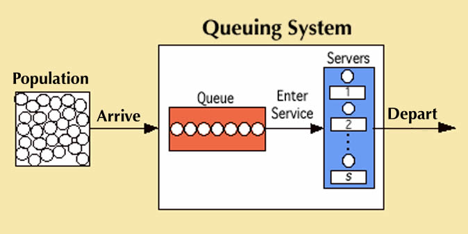
The input source, also called the calling population, is the collection of customers providing inputs to the queuing system. We assume for this model that the calling population is infinite, that is, the rate of arrivals into the system is unaffected by the number already there.

A queue discipline defines the rules by which customers are selected for service. A common discipline, assumed here, is first-come-first-served. Service is provided by one or more servers (or channels) operating in parallel. The servers may or not be identical.

The queuing system is the combination of the queue and the service channels. For this model, we assume that the total number of customers that can be present in the system is limited to some maximum number. That is, the size of the queue is finite and limited by the maximum number in the system less the number of servers. When customers arrive and find the queue to be full, the customer does not enter the system and does not receive service.

The state/event model is illustrated by the network below. The states are the nodes and the number in each circle is the number of customers in the system. The event of an arrival indicated by a, adds 1 to the number in the system. The number of servers is s. When the state number is less than or equal to s, all customers are in service and there is no queue. When the number in the system exceeds s, a queue forms.The service event, indicated by d, reduces the number in the system.

The queuing model is really a birth-death model with prescribed birth and death rates that depend on the number in the system.

Data for the CTMC

We create the model by choosing Data from the DP Data menu. The model selection dialog is presented. Here we consider the Queue model.

The program allows three types of models, the two kinds of Markov Chains (DTMC or CTMC) or the stochastic programming model (MDP). There is no DDP model provided for queuing. The selection at the left creates the CTMC model.

The are no decisions for the Markov chain models. The MDP models include the action of adding or removing a service channel. This could be an important issue in many queuing systems.

The two parameters of this system are the maximum number in the system and the number of servers. We have chosen small numbers for these parameters to simplify the presentation of the example. The numbers can be changed on the worksheet. When the Different Channels box is checked, each service channel will have its own rate of service. With the Common queue type the customers all wait in the same queue. The alternative of having separate queues is not modeled at this time.

By checking the Random Problem box, the server rates are randomly generated when the servers are different.

The data form is created by the add-in and placed on a worksheet. The model worksheet is built by clicking the Build Model button. The model is linked by formula to the data worksheet, so the model can be adjusted by simply changing the data. The titles in column D describe the data items.

The CTMC has two kinds of costs, cost rates that occur continuously over time and discrete costs that occur at specific times. The CTMC model uses both. Cost rates refer to states while discrete costs refer to transitions and actions. For this model we set the holding cost rate in E12 and the cost rate for open channels in row E14. The arrival and departure costs occur at discrete times of arrival or departure.

Notice that the data gives the service rate per channel, rather than the rate of departure. The latter depends on the number in the system.

Data for the DTMC

The DTMC model requires event probabilities rather than event rates, so to approximate the exponential distributions of the continuous process we define a time interval that should be small relative to the rates. We use 0.01 for the example. In general:

Event Probability = (Event Rate)*(Time Interval)

For the example with a time interval of 0.01,

Arrival probability = Arrival Rate*(Time Interval) = 0.1

Service probability from an occupied channel = Service Rate*(Time Interval) = 0.06

The time interval chosen must be small enough that probabilities are considerably nearer to 0 than 1. The discrete approximation assumes that only one event occurs in an interval. The assumption is better with very small intervals.

The per period costs and probabilities are computed in the cells colored yellow on the data form. The holding cost, cost for open channels, and discount rate are computed from the continuous cases by multiplying the associated rate values of the continuous case by the time interval. If the time interval is changed, the corresponding costs and probabilities change automaticaly.

Data for the Stochastic Dynamic Programming (MDP) Model

This model adds decisions to the DTMC. At each state, the number of open channels may be increased by 1, decreased by 1 or left the same. This addresses an important operating decision for many queuing applications.

Data on rows 15 through 18 describe features related to the decisions. E15 specifies the minimum number of channels and E16 specifies the maximum. The one time cost of increasing the channels by 1 is in E17, and the cost of decreasing the channels is in E18. Cell E19 is the cost rate for open channels. When a channel is closed the cost rate is 0.

Of the three options considered here, the MDP model is the only case that requires a dynamic programming solution approach. The others can be solved with either the Markov Analysis add-in or the DP Solver add-in.

Model with Different Service Rates

Clicking the Different Channels box on the queue dialog reveals the data structure below. The figure shows the CTMC data. The data now provides a vector of service rates, one for each server. The vector has the dimension of the maximum number of servers. The number of channels can be changed in E6, but it should be less than the maximum number of channels. There is a DTMC version of this model, but the MDP model is not extended to this case.

Summary

The Queue data option provides several different queuing models. Once the model is constructed different cases can easily be created by simply changing the numbers on the data form.