 |
The models for this section are
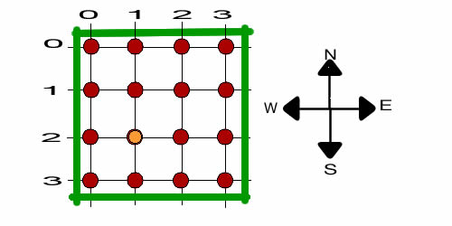
all based on grids as illustrated in the picture. The example
has two dimensions, but the add-in handles an arbitrarily number
of dimensions. In each dimension two movements are allowed.
One increases the value for a dimension, while the other deceases
it. For the example the dimensions are N/S and W/E, and the
movements are N, S, E and W. The coordinates of a point
in the region represents a state. For illustration consider
the point to be the location of a walker on the grid. The figure
shows the location of the walker at point (2, 1). Note that
the N/S dimension is first and the W/E dimension is second
in the state dimension. The N/S coordinate increases with a
move to the south and decreases with a move to the north. The
W/E coordinate increases with a move to the east and
decreases with a move to the west.
The walker is moving around the grid in steps parallel to
the boundaries. The boundaries are the green lines in the figure.
In every state, movement is possible in each direction as long
as the point is not on one of the boundaries. We recognize
two different boundary effects, the balk and the wrap. We first
consider the balk. When the walker tries to move outside a
boundary, he balks and does not move at all.

There are several different models available
from the walk option. The current version of the program
allows CTMC and DTMC models with the same or different probabilities
and costs on each grid line. These models involve probabilities
and no decisions. They are generally called the random
walk problem. There
is a deterministic dynamic programming (DDP) option that considers
actions, but no probabilities. The DDP seeks the shortest paths
from each state to one or more terminal states. An MDP option
that combines actions and probabilities. There are a number
of practical applications of the model.
This page describes the data structure
used by the program, the basics for the CTMC model, and some
sample solutions for small problems. For this first example,
we assume that each state has the same probability of movement
in each direction. There is a cost for traversing a grid line
and a second cost for balking. |
Data for the CTMC |
| |
We create the model
by choosing Data from the DP Data menu. The
model selection dialog is presented. Here we consider the Random
Walk model. |
| |
|
The program allows three types of models,
the two kinds of Markov Chains (DTMC or CTMC). the deterministic
dynamic programming model (DDP), and the Markov Decision
Process (MDP) model. The selection at the
left creates the CTMC model. |
|
| |
|
The two parameters of this
system are the number of grid dimensions and the
number of final states. Neither of these numbers, nor the
name can be changed after the model is constructed. The Boundaries options are wrap and balk. A
balk restricts movement at the boundary at a cost. For
the wrap option a movement past the boundary results
in a transition to the corresponding state at the opposite
boundary.
By checking the Make Random Problem box,
the transition rates and cost parameters are randomly generated.
The initial size of the grid is in the field
at the bottom. The example pictured above has a size of
4 in both directions. The value of each dimension ranges
from 0 to 3. The dimension sizes may be changed on the
data worksheet.
The data form for the example is below. |
|
| |
|
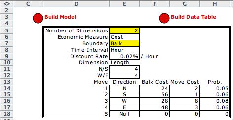
The data form is created by
the add-in and placed on a worksheet. The yellow cells
can not be changed, while the white cells can be modified
to suit the modeler. This model shows the balk and move
costs and the transition rates. The values are assumed
to be the same for all states.
The model worksheet is built by clicking
the Build Model button. The model is linked
by formulas to the data worksheet, so the model can be
adjusted by simply changing the data. The titles in column
D describe the data items.
|
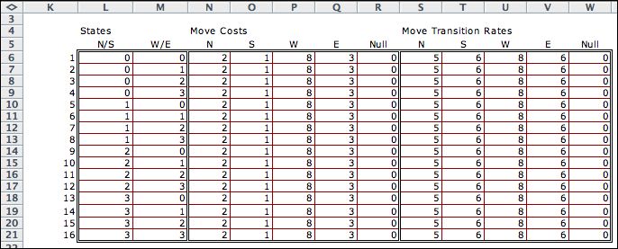
| A Build Data Table button constructs
a table on the page that allows the costs and rates to depend
on the state. The default table information comes from the move
cost and rate columns.
The balk costs are the same for all states. Changes in the
table will be reflected in the model. |

|
| |
Clicking the Make Model button
on the top of the data worksheet, calls the DP Models add-in
to construct the model worksheet. We discuss the model on the
next page. No direct interaction with this model is necessary
to solve the walk problem. All the data is on the data
worksheet.
Clicking the Transfer to Markov
Analysis button on the model worksheet creates a CTMC
matrix model. |
| |
|
| |
The transition costs appear in the
economic matrix. |
| |
|
| |
The steady-state solution is shown
below. The expected transition times are equal for all states,
because all states have the same transition rates. |
 |
Data for the DTMC |
|
|

|
The DTMC data is similar to the
CTMC data except that move probabilities are required
rather than move rates. The model for this problem can be solved
by either the DP Solver or the Markov Analysis add-ins.
The data on the left corresponds to an approximation of the
CTMC solved above with a time step of 0.01 hours. The probabilities
are computed as the move rates multiplied by the time step.
The discount rate has also been adjusted for the time step.
The probabilities do not add to 1 because the add-in assumes
that all unspecified probabilities are included with non-move
probability.
Clicking the Build Model button creates the model
worksheet and clicking the Transfer to Markov Analysis button
on that worksheet constructs the matrix model below. |
| |

|
| |
The transition matrix for the DTMC
has the same off-diagonal costs as the CTMC. The diagonal costs
are different because the transitions are governed by probabilities
rather than rates. |
| |
|
| |
As expected the steady-state
probability solution for the discretized problem is similar to
the steady-state-step probability solution obtained for the CTMC.
The expected NPW values are approximately the same. The average
cost per period for the DTMC is very close to the average cost
rate of the CTMD multiplied by the step size. |
 |
| |
The solution obtained
from the DP Solver add-in is the same. |
| |
|
Data for the Deterministic Dynamic Programming
(DDP) Model
|
| |
|
This model has no probabilities, but only costs. A single
terminating state is provided by the data with a cost of -1000.
The goal of the optimization is to minimize the total solution
cost. This is the shortest path tree problem, terminating at
a single state. For the example, the final state is (3,0).
We have zeroed the balk costs, so only the move costs are relevant.
Since the cost is negative at the terminal node (actually
a reward), the solution will seek the set of shortest paths
from every node to (3,0).
The DP Solver model for this problem is shown below. The policy
specifies the action to be taken from each state. The solution
for state 1, (0, 0) is identified by the outlined rows. Given
the simplicity of the data, this solution is not surprising.
This problem is more interesting when the move costs depend
on the state. The required data form is easily constructed
with the Build
Data Table button.
By providing more than one exit state, the solution will
determine the shortest path forest with as many trees as exit
states.
|
| |
|
| |
 |
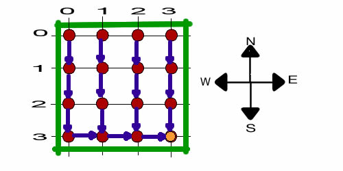
The figure shows the solution
to the problem obtained from the DP Solver add-in. Every initial
state defines a path to the finish state. For example, starting
from (0,0) the path moves south for three steps to state (3,0).
Then at (3,0) the path turns east for three steps to finally
end at (3,3). |
Summary |
| |
The Random Walk data
provided by the add-in is quite general and can be adapted
to a variety of applications. |
| |
|


