For the deterministic dynamic programming model we drop the random from the title, because the moves are not random in this case. The walker must follow a path to a designated terminal node. The goal is to find the path that is least expensive. The problem might be more accurately called the grid-walk problem because the walker is restricted to the grid lines.

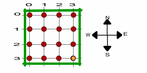
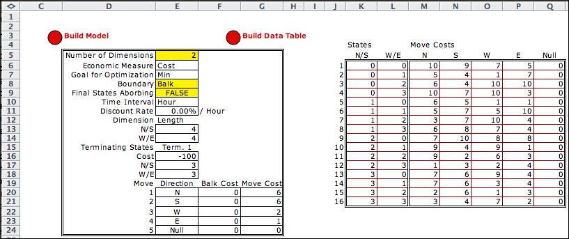
This model has no probabilities, but only costs. A single terminating state is provided by the data with a cost of -100. The goal of the optimization is to minimize the total solution cost. This is the shortest path tree problem, terminating at a single state. For the example, the final state is (3, 3). We have zeroed the balk costs, so only the move costs are relevant. Since the cost is negative at the terminal node (actually a reward), the solution will seek the set of shortest paths from every node to (3, 3). To illustrate a matrix presentation of the move costs, we have used the Build Data Table option. The numbers shown in the table were randomly generated. The model uses the tabular data rather than the move costs in column G.

States and Action

To create the DP Model, click on the Build Model button. Rather than the event element of the Markov Chain, the deterministic DP model has an action element. The decision moves the walker from one state to another. The state shown below is (2, 1) and the current action is to move south. The action element has a cost, but not a probability. The cost in cell M21 is a reference to the data table that uses the state index in E14 and the move index in K14 to select the appropriate cost.

The model has a new component, the State Subset. We use the first subset to define the terminating state. The first subset is true only for the state (3, 3). This is designated as a terminal state, and the cost of encountering the state is -100. We use this negative cost to specify an award for reaching the terminal state. It is also defined as an Exit state. When this block is encountered during the enumeration, no transition is required because the transition is automatically set to the final state. It is necessary to include the second subset so that the other states will be included in the analysis.

Enumeration

The state list is similar to the Markov Chain model, but a final state (state 16) is included. Whenever one or more states are indicated as exit states, the final state will be added to the list.

The action list has four alternatives. The cost column is irrelevant to the model, since action costs are determined by a matrix. We will see the link costs as decision costs for this model.

Decisions

For the DDP problem, transitions are shown in the Decision List. A decision is described by a state and an action. The transition blocks are similar to other models of this class with the blocks of two types. The first four blocks describe balk or wrap transitions. A balk occurs when a move is taken in a direction restricted by a wall. With a balk the state does not change. This is illustrated by the first decision in the in the Decision List where the move north is restricted. The second four transition blocks describe moves that change the state. The second on the list is an example. The first 28 decisions are shown below.

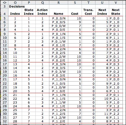
The last few decisions on the list illustrate an exit state. Row 61 shows the transition to the final state with the associated transition cost. The final state is added as state 17.

When the wrap option is in chosen a movement toward the boundary is not limited. An action moving toward the boundary results in the walker moving to a state adjacent to the opposite boundary. If the wrap option had been selected for this example, the action of moving north from state (0,0) results in a transition to state (3,0).

Call Solver

The DDP model uses the DP Solver to find solutions. The solution is below with the optimum recovered for state 1.

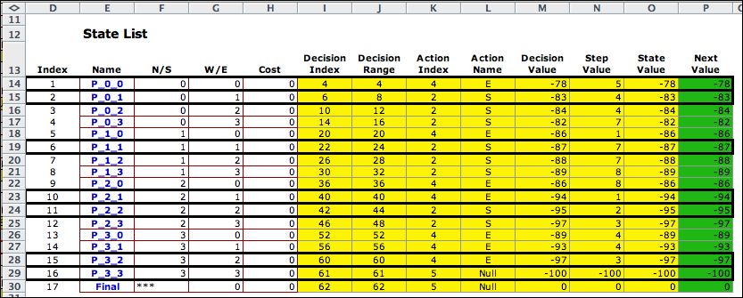
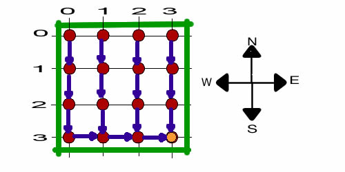
Column L gives the optimum solution for each state as pictured below. The collection of actions is the optimum policy. The solution is the shortest path tree rooted at (3,3).

Summary

This page has demonstrated the DDP model for the grid walk problem. The DP Data add-in constructs a table holding the data. By clicking the Build Model button on the data worksheet, the DP Models add-in constructs the model worksheet and fills it with the constants and formulas that implement the model. By clicking the Transfer to DP Solver button, the DP Solver add-in creates the solution worksheet and transfers the information from the list worksheet. All three add-ins must be installed for all the steps to work.

The solution algorithm implemented by the Value Iteration method does not require that the solution determine a tree. Every state has one of the four movements assigned, but there is nothing that restricts some subset of the states to be connected by a cycle of links. This will happen if the sum of the costs around some cycle is negative. In this case the solution does not converge. The values of the states on the cycle are unbounded from below. If there are no cycles with negative total cost, the state values will converge and the optimum policy will describe a tree.