 |
The DDP model of the resource
problem has only states and actions. No events are required
because there is no uncertainty in this model. We use the two
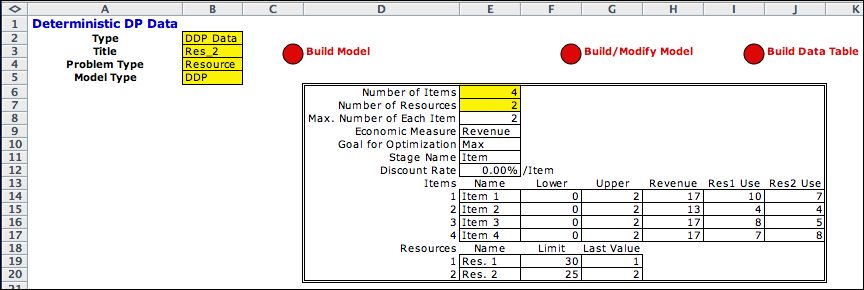
resource model as an illustration. The data for this model
is shown below. |
 |
States and Action |
| |
This model uses the Stage feature.
We need two state variables to represent the two resources.
The stage indicates the item number. We define
stages
because each item has different parameters. When the stage
feature is used, the first state variable is devoted to the
stage number. In the example stage variable starts at 1 and
goes to 5. The first four values represent the four items of
the problem and the fifth is used for terminal states. The
second stage variable indicates the amount of the first resource
used. The third state variable indicates the amount of the
second resource used. The initial state, S(1,0,0)
indicates that the action taken is to choose the number of
item 1 to include when no resources are currently used. Maximum
values of the states are passed from the data worksheet. When
the data is changed, the upper bounds on the state variables
are also changed. |
| |
|
| |
The action is to choose the number of items
of the type specified by the current state. The number ranges
from 0 to the maximum number of items given in the third row
of the data form (Max. Number of Each Item). The maximum
values for the individual items
is limited in the Decision blocks discussed later
on this page.
The action is evaluated in cell N21. The number in this cell
is drawn from the revenue data table using the Excel Index
function. |
State Subsets |
| |
State subsets are placed immediately below
the state and action definitions. The first subset describes
the exit states. Note that the lower and upper bounds in cells
F39 and F40 are both set to the maximum of the first state
variable. States with the item number of 5 are terminal states
and transitions are created to the final state through the
TRUE value in R39. The revenue in R38 is computed as the value
of the resources left over. The resources left over are computed
for convenience in row 41. Of course, the initial state S(1,0,0)
does not satisfy the condition of this state subset, so the
entry in R37 is computed as FALSE.
The second state subset includes all states. The second subset
includes all the terminal states, but the first subset
is chosen over the second when both are feasible. |
 |
| |
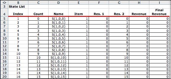
The enumeration process finds all combinations
of three state variables. The number of combinations is equal
to the product of the ranges of the three variables, 5*31*26
= 4030. The last state is the final state for a total of 4031. |
| |

.

|
| |
The action list has three alternatives. The
cost column is irrelevant to the model, since action costs depend
on the combination of state and action. |
| |

|
Decisions |
| |
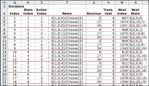
Decisions describe combinations of states and actions.
The boundaries on the decision block for the first state variable eliminate
terminal states (state 1 equal to 5). These
are defined as exit states in the state subset blocks and there
is no need to repeat them here. The decision maximum in M58 is
passed from the item limit on the
data worksheet. Individual
items may have smaller limits than the overall maximum. The revenue cell
holds the value computed on the revenue table on the data worksheet.
Thus it reflects
both the
item state variable and the action. |
| |
 |
| |
There are 6895 feasible decisions
for this example. |
| |

.

|
Call Solver |
| |
Clicking the Transfer to DP
Solver button on the top of the model worksheet calls
the DP Solver add-in to construct the solver model and transfers
the list information to the form. Click the Solve button
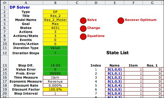
to perform the DP algorithm. Only Value iterations
are available for the DDP model. The
upper left corner of the worksheet is shown below after the
optimal
solution has been found. Seven value iterations are required. |
| |
 |
| |
Click the Recover Optimum button
and choose the initial state. The default value is state 1. The
optimal states are shown in the next figure. The list is below
the state definition on the worksheet. The system starts in
state S(1,0,0). The optimum action is choose none of item 1 and
the state moves to S(2,0,0). The optimum action in that state
is to choose two of item 2. This moves the system to state S(3,8,8).
The 0 action at state S(3,8,8) leads to S(4,8,8). The 0
action at state S(4,8,8) leads to S(5,8,8). This is an exit state
so finally the system moves to the final state and the optimum
sequence is complete. |
 |
| |
|
Summary |
| |
The problem of selecting
alternative activities that use limited resources is
a classic problem of operations research. The dynamic programming
solution approach suffers from the curse of dimensionality. The
number of states and decisions grows rapidly with the size
of the problem.
DP handles problems with separable nonlinear objective function
and resource requirement functions with little variation of
the models described here. Also, problems with uncertainties
regarding resource usage can be addressed with
the addition of events to the model. The resulting model is
a MDP model.
Deterministic resource allocation problems are more readily
handled by mathematical programming. Problems with many activities
and resources can be easily addressed. Separable
nonlinear terms in a math programming model are more difficult to
formulate but well within the capacities of modern computational
systems. It more difficult to add the uncertainties to the
math programming model, and DP may well have an edge for this
kind of problem. |
| |
|


