|
|
 |
Dynamic
Programming
Examples |
 |
-
Doors Problem |
 |
The inspiration for this MDP
version of the Random Walk problem is the paper Combinatorial
Design of a Stochastic Markov Decision Process, by Nedialko
B. Dimitrov and David P. Morton (in Operations Research and
Cyber-Infrastructure, M.J.\ Saltzman, J.W. Chinnek and B.\
Kristjansson (eds.), Springer, New York, 2009, 167-193). It
is the MDP option of the Random Walk problem described
in the DP
Data section of
this site.
One
of the problems considered by this paper is described by the
authors in this slightly modified quotation.
| Suppose an individual moves randomly on the grid network
depicted in Figure 1.1 (repeated below). The
top-left cell (northwest corner) and the bottom-right cell
(southeast corner) are special. We seek
to guide the individual to the northwest corner, but he
vanishes from the grid if he first reaches the southeast
corner. The set of grid cells, i.e., nodes in the individual’s
spatial network, form the state space. There
are five actions available in each cell: do nothing,
close a one-way door blocking the north exit, the south
exit, the east exit, or the west exit. If we do nothing,
the individual has a 1/4 probability
of transitioning to the adjacent cell to the north, south,
east, or west in the next time period. If we
close a one-way door blocking one of the cell’s exits,
the individual has a 1/3 probability of exiting to
each of the remaining three neighboring cells. The doors
are one-way since they block movement
out of, but not into, the cell. The special cells are different:
If the individual reaches the northwest
corner, or the southeast corner he departs the grid in
the next time step, regardless of the action we
take. In the former case we receive a unit reward. The
one-step reward for the latter case, along
with that of all other cells, is 0. As a result, the goal
is to maximize the probability the individual
reaches the northwest corner prior to reaching the southeast
corner and vanishing. Equivalently,
the goal can viewed as “protecting” the southeast
corner, i.e., as minimizing the probability the
individual is allowed to transit into that cell. |
The add-in does not solve exactly the problem considered in
the paper, and the paper goes far beyond the simplest of the
problems considered here.
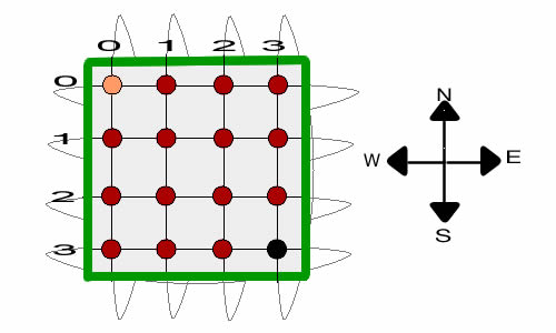
The MDP model adds the blocking
action to the Markov Model of the random walk problem. At each
state, we allow the action of blocking movement in one of the
directions. The figure below illustrates the problem. For this
case we assume that the grid lines wrap. When the
walker reaches one of the boundaries and attempts to move beyond
it, the walker goes to the opposite boundary. For example with
the walker at (0, 1) and attempts to move north, he will find
himself at the next step at (3, 1). The wrapping is illustrated
by the oval shapes that appear to go behind the grid.

Two states are designated as final states, (0,0) and (3,3).
If the walker wanders to state (0,0) indicated by the gold
color, we win a reward of $1 and the walker leaves the grid
and goes to a final state that is external to the grid. If
the walker wanders to state (3,3) indicated by the black color,
we win no reward and the walker leaves the grid and again goes
to the final state. This is called a transient MDP because
the walker will eventually leave the grid.
The actions of the MDP involve closing the door against movement
in one of the four directions. In each state we may decide
to restrict movement or not. If restricted, we must choose
the north, south, west or east direction. We combine the decision
to restrict with the four movement directions by including
the null decision
along with the four directions. If not restricted, the walker
moves in the four directions with equal probability of 1/4.
When the walker is restricted, the probability of moving in
the restricted direction is 0, and the probability of moving
in each of the other directions is increased to 1/3. Doors
are one-way in that they only restrict movement from the state
restricted, not from some other state moving into the state
restricted.
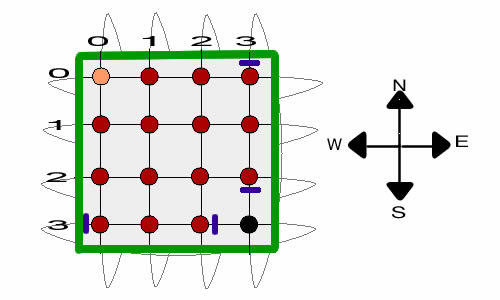
We illustrate a door by the short blue line close to the
node representing the state. The solution shown has the black
node entirely sealed off. All avenues of direct movement into
the black node are blocked. Note that all four doors of the
solution are not simultaneously present. A door is closed only
when the walker is in the associated state.

|
Data |
| |
|
The dialog for the MDP version
of Random Walk data type is shown at the left.
Only the Final option is allowed for exit states.
For this example we choose the wrap option for
boundaries, and specify 2 as the number of exit states. |
|
The data form for the Doors problem shows
the data that is fixed for the model with yellow cells.
The decision to place a door at a cell is called the
blocking decision and this form has data defining the
cost of placing the block.
We have filled in the specific data for the problem.
Note the prize for the final state (0,0) is set to 1.
In contrast to the problem presented in the paper we
indicate a block prize of -0.001. This is a small penalty
placed on using a door. Otherwise, there are many alternative
optimum solutions to the problem. The small
penalty will encourage a solution with as few doors as
possible.
There are five moving decisions, one for each direction
and one for the no-move option. To correctly reflect
the doors problem the probability of the null
move must set at 0. |
|
States |
| |
Clicking the Build Model button
creates a worksheet for the model. The MDP model has
all three elements, States, Actions and Events.
The following discusses each element and illustrates the associated
lists that define the problem for the DP Solver. |
| |
|
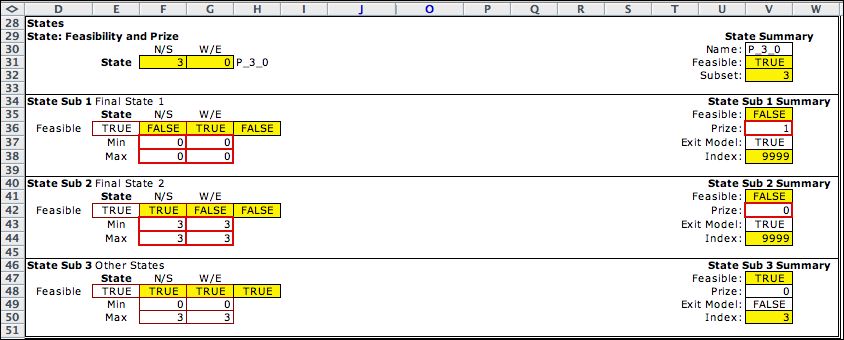
The state space is identified by enumerating
all integer indices from 0 to 15 in cell E14. We choose
the index 12 and the resultant state (3,0) for illustration. |
|
The state list, obtained by enumeration, has sixteen
states representing the nodes on the grid and one additional
state called the final state. This new state
is included for any problem that has exiting states designated
as a final state. |
The final states are designated in the state
subset range of the worksheet shown below. Here states
(0,0) and (3,3) are defined as exit states with the word
TRUE in V37 and V43. The prize of 1 for exiting
at state (0,0) is in V36 of the first subset. The
third subset includes all the non-exit states.

|
Actions |
| |
|
The five actions are identified with the
integers 1 through 5. For example, the integer 4 is the
block action of closing a door to the east. The penalty
for using the blocking action is in M21. The cell holds
a formula that links to the corresponding value
on the data worksheet.
The blocked probability cell in M22 is transferred
from the move probability cells on the data worksheet.
The value shown is the move to the east probability. |
|
The action list is obtained by the
enumerating the actions. |
|
Events |
| |
|
There are four move events. The interesting
thing about this problem is the computation of the event
probability in cell R22. Cell R22 holds a formula that
sums P22 and Q22. Cell Q22 holds the value of the move
probability transferred from the data worksheet.
Cell P22 holds the contribution from the block decision.
When it is the same as the move event, then the negative
of the blocked probability is entered in P22
so that the net probability is 0. |
|
When the move is different than the block decision as
is shown at the left, 1/3 of the blocked probability is
placed in P22. The net probability of the westward move
is the desired value of 1/3. The evaluation of P22, Q22,
and R22 are all accomplished through Excel formulas. The
results are valid with any valid move probabilities entered
on the data worksheet.
The formula in P22 is the only reference to the action
required on the model worksheet. |
|
The event list is obtained by the enumerating
the events. |
|
Decisions |
| |
The decision list is created by enumerating
all states and all actions. Only feasible combinations are
included. There is only one decision for state (0,0). Since
(0,0) is final state, no actions are enumerated and the action
in state (0,0) is specified as Null. The prize for
state (0,0) as well as the penalties for all blocking decisions
are in column Z. There are no decision blocks for this model,
so the list is a straight forward enumeration of all state/action
options, except for states (0,0) and (3,3).

The last few decisions are shown below to illustrate the transition
at the exit state (3,3). Row 72 shows the transition to the
final state with the associated prize. The final
state is in row 73.

|
Transitions |
| |
The transitions are defined by the transition
blocks of the model. Although the actions are included in the
transition block definition, the same transition blocks are
used as were used in the Markov Chain models. The actions play
no role in the transitions except in the determination of the
probability of transition in the event description.
These are transferred to the transition blocks and ultimately
appear as the transition probabilities in column AG.
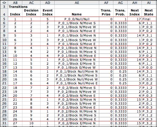
Each decision has a set of transitions, and each member of
the set is the result of a different event. For the example,
the first row indicates the transition from state (0,0) to
the final state. Transitions 2 through 4 are for the action
of blocking north from state (0,1). The move north
event is not shown because its probability is zero. The other
three move options each have a probability of 1/3. Transition
5 illustrates a wrap transition where the state (0,1) moves
to state (3,1) with a northward move. Only the null action
has four move events, each with probability 1/4.

There are 227 transitions for the model. The
transition from (3,3) to the final state is 226. The final
state (state 17) is an absorbing state with 0 transition
cost and probability equal to 1.

|
| |
Click the Transfer to DP Solver button
at the top of the models worksheet to automatically build the
Solver model and fill the solver worksheet with the five
lists shown above. The lists of states, actions, events,
decisions and transitions comprise the input data for DP
Solver model. The solution obtained is described on the next
page. |
| |
|
|


