A network flow solution algorithm is provided by the Network Solver add-in (net_solver.xla). The Excel Solver actually solves network problems by solving the underlying linear programming problem. Network algorithms are generally faster than linear programming algorithms for solving problems that can be modeled entirely as networks. This algorithm is used when the user chooses the Jensen Network Solver for either the Network or Transportation models of the Mathematical Programming add-in. The add-in must be installed prior to clicking on the Solve button for either case. The add-in works for linear problems that may or may not have integer variables.

There are no built-in limits for model size. Arrays are dimensioned automatically. For large problems, excessive memory requirements may cause the program to crash or computation time may be large.

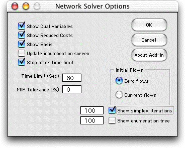
The Jensen Network Solver add-in puts an item on the OR_MM menu: Network Solver. Choosing this item presents the dialog form shown below. The options on this dialog control the Jensen Network Solver. These options are particularly useful for the student interested in the procedures used in network optimization algorithms. The following describes the several categories of options appearing on this dialog.

Note that the Network Solver add-in only works for models constructed with the Math Programming add-in. A valid network model must be on the active worksheet when the Network Solver menu command is selected.

The solution parameters specified on this dialog are stored on the worksheet in column A starting at row 2.

Solution Display Options

These options print information on the problem worksheet or on a separate worksheet. The displays are useful for debugging algorithms, learning the principles of the algorithms and sensitivity analysis.

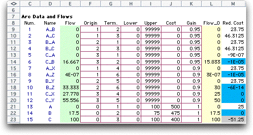
The figure below shows the worksheet for the Power example. The reduced costs are shown on the arc display in column M.

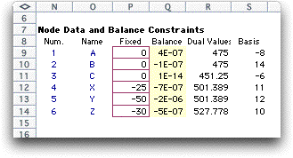
The dual variables basis tree information is shown on the node display.

The figure below shows the artificial arcs added prior to the beginning of the network simplex iterations. There is one artificial arc for each node. The computer adds three nodes to the original 6 nodes specified in the model. Node 7 is a super source node, node 8 is a super sink node, and node 9 is called the slack node. Four new arcs, 16-19, are added to connect the slack node to the super source and supper sink. The artificial arcs begin at arc 20.

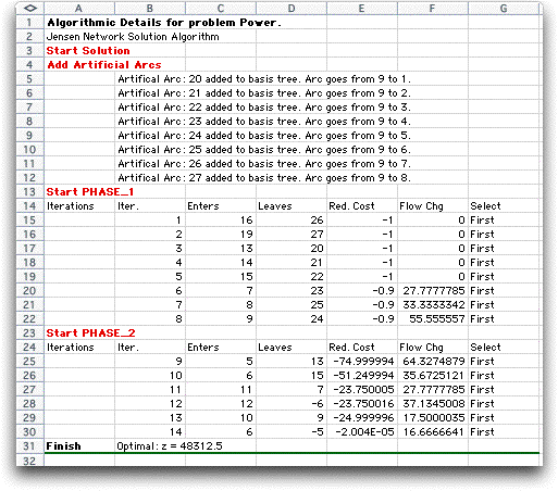
The simplex iterations first drive out the artificial arcs from the basis during phase 1. The phase 2 iterations move toward the optimum basis obtained at iteration 14.

The enumeration tree is obtained for generalized problems (all gains not 1) when some arcs are required to have integer flows. The output is similar to that obtained with the Jensen LP/IP solver.

Algorithm Control Options

• Initial Solution: Two different starting strategies are available. The first option starts with all arc flows equal to zero and an all artificial initial basis. The second strategy gathers the initial flows from the values shown on the worksheet. If a basis is displayed, the arcs listed are used as the initial basis. The algorithm starts with these values for the flows and the basis. The advanced start option will result in fewer iterations when only slight modifications are made to the network model.
• MIP Tolerance: When solving all integer or mixed integer programming problems, vertices of the enumeration tree are fathomed when the relaxed solution objective is less than (for a maximization problem) than the incumbent solution. This tolerance makes the fathoming test a little easier by fathoming the vertex if its relaxed objective is within x% of the incumbent solution, where x is the number entered in this field. The solution may be found with fewer iterations and less time when this value is greater than 0. When the tolerance is other than 0, however, there is no guarantee that the optimum solution is obtained. It is a guaranteed that the solution is with x% of the optimum. The Excel Solver has a similar tolerance specified in the Options dialog of the Solver.
• Time Limit: When solving all integer or mixed integer programming problems the process may take a long time. The program will stop when this time limit is reached. The user may give up at this point or continue the optimization. The Excel Solver has a similar time limit specified in the Options dialog of the Solver.
• Update Incumbent on the Screen: When solving all integer or mixed integer programming problems, the algorithm may find feasible solutions during the enumeration process. The feasible solution with the best value is called the incumbent solution. Although intermediate steps are not displayed on the model worksheet while the process continues, when this checkbox is selected, the display will be changed whenever a new incumbent is discovered. For later versions of this add-in the incumbents are displayed automatically.