|
|
 |
Random
Variables |
 |
Add Random Variable
|
 |
The game of Craps is
a popular gambling game. In this game, the player rolls
a pair of dice and sums the numbers showing. A sum of 7 or 11
wins for the player, and a sum of 2, 3, or 12 loses. Any other
number is called the point. The player then rolls the dice again.
If she rolls the point number, she wins. If she throws a 7, she
loses. Any other number requires another roll. The game continues
until the gambler rolls a 7 or her point number. We use this
situation as an example of a random variable. |
| |
 |
Simple probably analysis
determines that the sum of two standard dice is a discrete
random variable with integer values ranging from 2 through
12. The probability distribution of the sum is the triangular
distribution with a mode of 7. To define this distribution
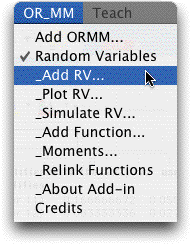
for subsequent computation, select the Add_RV item from
the OR_MM menu. The dialog box shown below opens. |
|
| |
|
| |
Sixteen
named distributions are available with one user defined distribution
and a general distribution. The option buttons at the left
select discrete distributions, while the option buttons on
the right select continuous distributions. An exception is General that
can define both continuous and discrete distributions. The
User distribution allows entry of a user specified discrete
probability distribution.
For the example we name the random
variable Dice, identify it as an integer triangular distribution,
specify its lower value, mode and upper value as 2, 7 and
12 respectively. The check boxes on the right of
the dialog, list optional information that will be shown
with the distribution.
One or more random variables must be
defined with the Add_RV option before any of the other programs
or functions may be used. The names for random variables
must be unique and not previously defined for the workbook.
The cell reference shown at the top of the dialog box is
the upper left corner of the worksheet range where the random
variable information will be stored. The value of this cell
is the reference to the cursor location when the dialog is
called. When the "Show Titles" checkbox is clicked,
the titles associated with the distribution parameters are
shown. When not clicked only the parameters are shown without
titles. The latter is useful when a series of random variables
are defined each with the same set of parameters. The other
checkboxes at the right specify that a series of computations
related to the random variable are to be presented along
with the definition. |
| |
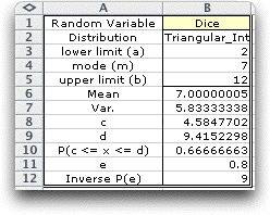 |
After identifying
a distribution and defining appropriate parameters,
the random variable information is placed on the worksheet
with the rectangular construction as in the example.
For each random variable defined in this manner, an
Excel Name is assigned to that portion of the array
that identifies the distribution type and parameters.
For the example the four cells headed by "Triang_Int"
are given the name "Dice". The name must obey
Excel restrictions on naming regions of the worksheet.
The random variable is referenced by this name. Any number
of random variables may be included on the worksheet. Once
defined, the distribution parameters may be changed by
simply typing a new value. Distribution parameters may
also be functions determined by other cells on the worksheet.
The example also shows additional
information regarding the random variable. These
are obtained with user defined functions, to be described
later.
The orientation of the distribution data is determined
by the Orient frame of the dialog. This example
has the vertical orientation. |
|
| |
The figure below shows
the same distribution with a horizontal orientation.

|
Replications |
| |
It is often convenient
to create several random variables simultaneously. To do this
select the number of replications to a number greater than
1. The figure below shows three Normally distributed random
variables in the vertical orientation. The three distributions
are differentiated by the _1, _2 or _3 added to their names.

The horizontal orientation for three replications is illustrated
below.

|
User Distribution |
| |
To
create a User Distribution, place the cursor on the
sheet where you want the distribution to appear. Choose Add
RV from the OR_MM menu, enter the name and number of cells
defining the distribution.
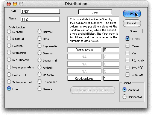
The resulting display with 5 cells is
shown on the left. Once the table is defined, the user enters
the several possible values of the random variable and the
associated values of the probability distribution as in the
example. The distribution values should sum to 1, however,
the functions will normalize the distribution if the total
probability is not 1. The table on the right shows three
user distributions defined by setting the number of replications
to 3. User distributions can only have vertical orientations. |
| |
|
|
General Distribution |
| |
It is often convenient
to construct a form first and add the distribution data later.
The General Distribution form is for this purpose.
To define the distribution click the General button.
The parameter values can be defined here, but it is convenient
to leave them at 0.
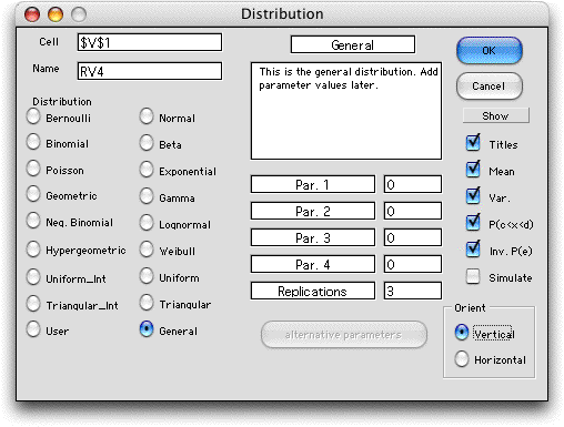
An empty form is created on the worksheet as
below.
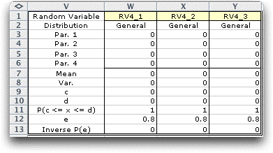
The columns can be used to identify any of the
named distributions listed on the distribution dialog. In the
following, Binomial, Beta and Exponential distributions are
defined.

It is unnecessary to enter the entire title of
the distribution because in all but two cases only the first
three letters are required. For example "Binomial"
could be entered as "Bin". The two cases are the
uniform-integer and triangular-it distributions. These are
identified by "uni-int"
and "tri-int", respectively. Other designations are
possible as long as the first three letters are "uni"
or "tri" and "int" appears in the name.
The titles in the left column do not indicate
the names of the parameters because each distribution has different
parameters. The parameters are entered in the cells immediately
following the distribution title in the order specified on
the distribution dialog. For example, the four parameters for
the Beta distribution are alpha, beta, lower
bound and upper bound. |
| |
|
|


