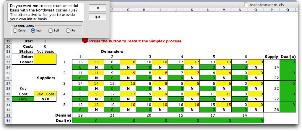
Return to Index
Operations Research Models and Methods
 
Models Section
Subunit
Teach Transportation Add-in
-Initial Tableau
The Tableau

When the start button is clicked, the add-in prepares the tableau form of the transportation simplex algorithm and places it lower on the worksheet. The simplex procedure requires an initial basis. The add-in presents the dialog below. The figure below shows the tableau and the dialog requesting basis.

northwest
 

The cancel option allows the student to provide his or her own basis. The tableau below shows the necessary data and computation information necessary to perform the primal simplex algorithm adapted for the transportation problem.

Each cell in the original data is represented by four cells in the tableau. The key is in the range A29:B30. The upper left cell, outlined and shown in white holds the transportation cost from the supplier to the demander identified by the cell. The cost data is transferred by formula from the data matrix in the rows above this display. The upper right cell holds the reduced cost, computed from the dual variables and the original arc costs. The lower left entry, in green, shows the flow assigned to the cells. Initially these values are zero. The lower right entry holds the letter N or B, indicating whether the cell is not basic (N) or basic (B). To begin the simplex method an initial basis must be selected.A basis is defined by placing a capital B in each of the basic cells.


Northwest Corner Rule

  The easiest basis is the one constructed by the Northwest Corner rule. The program constructs this solution automatically. The figure shows basic cells with the letter B and colored red.
northwest corner solution
 

The Northwest corner solution assigns flow to cells starting in the upper left corner. As each cell is considered, flow is assigned to use up all of the supply for a row or all the demand for a column. A complete description is in the textbook. The graphic shows the feasible flow that is determined by the Northwest Corner rule. The flows appear in the green cells.

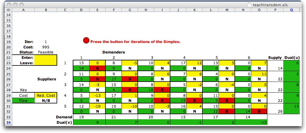
The dual variables u and v shown as the right most column and bottom row, respectively. The reduced costs are in the yellow cells.

The dual variables are associated with the rows and columns of the tableau. They are assigned so that the reduced costs of all basic cells are zero.

The formula for the reduced cost is

d(i,j) = c(i, j) - u(i) - v(j).

In this formula, i is the index of the row and j is the index of the column. c(i, j) is the cost for the cell. u(i) and v(j) are the dual variables associated with row i and column j. This notation as well as the complete algorithm are discussed in the textbook.

One of the dual variables is arbitrary and we assign that one the value of zero. For the case shown, we have assigned the 0 value to v(3). Given the first assignment it is always possible to assign the others based on the requirement that the reduced costs for basic cells are 0. Once v(3) is assigned, then the values of u(3) and u(4) are determined by the expressions:

u(3) = v(3) + c(3,3) = 8

u(4) = v(3) + c(4,3) = 9.

The basic cells all have d(i,j)= 0, but the other cells take on positive or negative values. The condition for optimality for the transportation problem is that all cells must have nonnegative reduced costs. This is clearly not true for the tableau shown in the figure, because the solution is not optimum.

The next page shows how to iteratively change the basis until the optimum is determined.


Return to Top

tree roots

Operations Research Models and Methods
Internet
by Paul A. Jensen
Copyright 2004 - All rights reserved

Next Page