| Transportation Model
Definition Dialog |
 |
 |
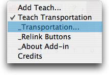
Create a model by selecting the Transportation command.
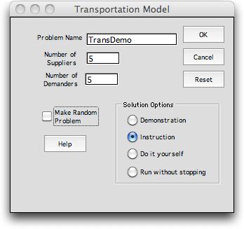
The add-in presents the dialog below with input fields
for the number of suppliers and demanders. Either input can
range from 3 to 10. A checkbox indicates whether random data
is to be supplied or the data form left with 0 entries. The
former case is useful for demonstrations or practice with
the transportation algorithm. The latter is appropriate if
the student has specific data to enter. |

The solution options provide different amounts
of information regarding the algorithm and different levels
of interaction with the student. As the algorithm progresses
it is possible to shift between the options.
- Demonstration: This option
provides a running commentary of the steps taken by the algorithm
as it progresses toward the optimum. The student is only required
to press a button from time to time.
- Instruction: With this option,
the student is required to make decisions about the process
taken by the algorithm. For example, the student must select
the cells to enter and leave the basis. A hint button provides
various levels of help. Pressing the hint button several times
eventually reveals the correct step. The program prevents
any serious deviations from the proper procedures.
- Do it yourself: Here the student has
the entire responsibility of directing the algorithm. No hints
or corrections are given. If the student is hopelessly lost,
it is possible to shift to the Instruction option.
- Run without stopping: Here the algorithm
is allowed to run to the end without commentary or interaction.
The entry for delay controls the speed of this option. The
program pauses for the specified number of seconds at each
stopping point. An integer number of seconds should be entered
here. Once this option begins, the algorithm runs to completion.
|
The Example Problem |
 |
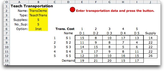
The figure below shows the transportation data form constructed
by the add-in. Data has been entered for the example of this
section. The yellow region in column B holds information
necessary for the program. This information should not be
changed by the student. Buttons control the progress. Click
on the Start button when the data is prepared.

|
 |
The transportation algorithm requires a balanced
problem in which the total supply equals the total demand. Our
example does not satisfy this requirement in that the supply
exceeds the demand. The program presents the dialog below prior
to addressing the situation. |
 |
|
 |
With a response of OK, the add-in creates a
dummy demander that has a demand equal to the excess supply.
Cell costs are zero in the new column. Flow assigned to the
dummy column represents supply that is not shipped. The new
model is shown below. |
 |
|
| |
The model is now complete.
The remainder of the pages in this section describe the primal
simplex applied to the transportation problem. |
| |
|


