|
|
|
|
Investment
Problem
|

|
DP
Finish |
|
|

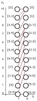
Figure 3.
Optimal decisions
for  =
7 =
7
|

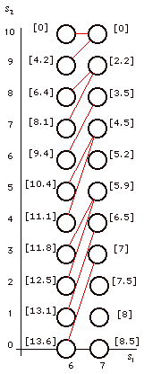
Figure 4.
Optimal decisions for
 =
6 =
6 |
|

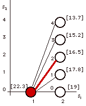
Figure 5.
Optimal decision for state (1, 0) |
The process continues until  = 1. At this point, the manager must make a decision
for opportunity 1. Since this is the first decision,
she knows how much of the budget is already spent. It
must be 0. Accordingly, we call (1, 0) the initial
state. Now it is possible to decide on the amount to invest
in opportunity 1 because the value of the remaining
budget for opportunities 2 through 8 is known. The decision
process associated with opportunity 1 is shown in Fig.
5.
The figure shows the four decisions leaving
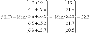
the initial state. The recursive equation used to determine
the optimal value and decision at (1, 0) is

with the optimal decision  =
2. =
2.
|
| Figure 6 depicts the collection of states used to solve
this problem. The set of all feasible states is called
the state space S. When we represent all the feasible states as nodes and all
the feasible decisions as arcs, the resultant network
is called the decision network of the problem.
Figure 6 is really a subnetwork for the investment problem
because it includes only the states that lead ultimately
to a state in the final state set and highlights only
the optimal decisions. A critical feature of the model
is that the return associated with each arc depends only
on the states at the two end points of that arc.
The procedure just described has uncovered
the path through the decision network with the largest
total return. For the investment problem, this path
starts at the initial state (1,0)
and terminates at the final state (9,10).
It is marked by heavy arcs and golden nodes in Fig.
6. |

Figure 6. Decision network with optimal solution
|
The algorithm computes the optimal decision leaving
each state. For the example, the decision in state (1,
0) is 2, leading to state (2, 2). The optimal decision
in state (2, 2) is 1, leading to state (3, 3), and so
on. The process of constructing the optimum decision
sequence is called forward recovery
since it begins in an initial state and moves in the
forward direction until a final state is reached. Table
3 lists the optimal decisions from one state to the
next.
|
Table 3. Path for the optimal
solution |
| |
State |
Decision |
Return |
|
Index |
|
|
|
|
|
1 |
1 |
0 |
2 |
22.3 |
|
2 |
2 |
2 |
1 |
16.5 |
|
3 |
3 |
3 |
1 |
14.7 |
|
4 |
4 |
4 |
2 |
13.2 |
|
5 |
5 |
6 |
1 |
9.4 |
|
6 |
6 |
7 |
2 |
8.1 |
|
7 |
7 |
9 |
1 |
2.2 |
|
8 |
8 |
10 |
0 |
0 |
|
9 |
9 |
10 |
-- |
0 |
The investor should invest $10 unit
each in opportunities 2, 3, 5, and 7; invest $20 million
in opportunities 1, 4 and 6; and make no investment
in opportunity 8. The entire budget has been spent
and there is no slack. The total annual return is
$22.3 million.
In addition to the path leaving (1, 0), it is possible
to identify an optimal path for every state by tracing
the optimal decisions from the specified state to some
final state.
The complete set of decisions is called a policy because it specifies an action for every state. The
amount of work required to determine an optimal policy
is proportional to the size of the state space. During
the solution process a simple problem, each with a single
variable, was solved for each state leading to an optimal
policy for all states. |
|
| |
|
|

