|
|
|
|
Investment
Problem
|

|
DP
Approach |
|
|
|
To begin, we ask the manager to decide on the amount
to invest sequentially. That is, we first ask her to
consider opportunity 1, then opportunity 2, and so on.
This is difficult to do in a way that maximizes the
total return. The manager notes that the more she invests
in opportunity 1, the greater the annual return. Consequently,
she might feel that a greedy approach is called for
-- one that invests in the highest possible level, 4
in this case. It should be apparent, though, that such
an approach may yield very poor results. Committing
a large portion of the budget to early opportunities
precludes potentially more attractive returns later
on. Instead, we ask the manager to solve the problem
backwards, starting with opportunity 8, then 7 and so
on until she makes a decision for opportunity 1. With
a little organization, we find that this procedure is
possible.
First we ask, how many units should we invest in opportunity
8? The manager responds that she cannot make that decision
unless she knows how much of the budget has already
been spent for the first 7 opportunities. Then, the
decision is obvious. For example, if all the budget
is spent by the previous opportunities, the investment
in 8 must be zero. If one unit of budget remains she
will invest 1 in opportunity 8 if the return exceeds
the 0.5, the value for leftover funds. In general, if
x units are already
spent, she can invest up to10 – x in opportunity 8. Of course when x is 5 or less, 4 units can be invested and there will
still be money left over. |

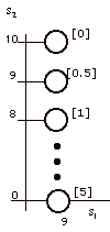
Figure 1.
States for s1
= 9
|
To formalize the dynamic programming
approach, we define states and decisions. A state is described by the opportunity index,  ,
and the amount already spent, ,
and the amount already spent,  .
The state variables are contained in the vector .
The state variables are contained in the vector  . .
We use  =
9 to mean that there are no more opportunities. For
this problem, we call any state that has =
9 to mean that there are no more opportunities. For
this problem, we call any state that has  equal to 9 a final state
because there are no more decisions in our sequential
process. The set of final states is F. For the investment problem

A final state has a value defined by
the final value function,
f(s).
For this problem, the final value is the annual return
of the funds not spent.

Graphically, we represent a state as
a node as in Fig. 1 where only the final states are
shown. The final state values are in brackets next to
the nodes.
|
|
Table 2. Optimal decision process
for opportunity 8 |
|
State |
Decision |
Decision objective |
Next state |
Next state value |
Total return |
Optimal decision |
Optimal return |
|
s |
d |

|
s' |
f(s') |
r(s, d)+ f(s') |

|
f(s) |
|
(8, 10) |
0 |
0 |
(9, 10) |
0 |
0 |
0 |
0 |
|
(8, 9) |
0 |
0 |
(9, 9) |
0.5 |
0.5 |
|
|
| |
1 |
1.0 |
(9, 10) |
0 |
1.0 |
1 |
1.0 |
|
(8, 8) |
0 |
0 |
(9, 8) |
1.0 |
1.0 |
|
|
| |
1 |
1.0 |
(9, 9) |
0.5 |
1.5 |
|
|
| |
2 |
1.7 |
(9, 10) |
0 |
1.7 |
2 |
1.7 |
|
(8, 7) |
0 |
0 |
(9, 7) |
1.5 |
1.5 |
|
|
| |
1 |
1.0 |
(9, 8) |
1.0 |
2.0 |
|
|
| |
2 |
1.7 |
(9, 9) |
0.5 |
2.2 |
|
|
| |
3 |
2.3 |
(9, 10) |
0 |
2.3 |
3 |
2.3 |
|
(8, 6) |
0 |
0 |
(9. 6) |
2.0 |
2.0 |
|
|
| |
1 |
1.0 |
(9, 7) |
1.5 |
2.5 |
|
|
| |
2 |
1.7 |
(9, 8) |
1.0 |
2.7 |
|
|
| |
3 |
2.3 |
(9, 9) |
0.5 |
2.8 |
|
|
| |
4 |
2.8 |
(9, 10) |
0 |
2.8 |
3 or 4 |
2.8 |
|
The computations for a particular state are shown by
the colored bands in the table. We see that a separate
optimization is carried out for each state s. The column labeled d shows all feasible
values of the decision variable. A value not in this
list would use more than the budget available. The decision
objective is the annual return for selecting the amount d. This value comes from Table 1. The column labeled
s' is the next state reached by making decision d while in state s. The next state is given
by the transition function
T(s, d). For this problem the transition function is

The value of the next state, f(s'), has already been computed and is shown in the next
column. The total return is the sum of the decision
return and the next state value and is the quantity
to be maximized.
For each value of s,
we compare the total returns for the different values
of d and choose the one that gives the
maximum. This is a simple one-dimensional problem solved
by enumerating the discrete alternatives. The optimal
decision is  , where the argument s indicates that the decision is a function of s. Finally the optimal return is the value f(s). , where the argument s indicates that the decision is a function of s. Finally the optimal return is the value f(s).
The computations are performed by solving
the following backward recursive equation.

It is a recursive equation because the
function f(s) appears on both sides of the equality
sign. We can solve it, only if we proceed in a backward
direction through the states.
|

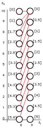
Figure 2.
States for  = 8 with optimal decisions
|
The optimal decisions for opportunity
8 are shown in Fig. 2 as the red lines between the
states. When a tie occurs it can be broken arbitrarily.
State (8, 6), for example, admits two optimal decisions
3 and 4. We have chosen 3 for the illustration. The
values for the states are shown adjacent to the nodes.
|
|
| |
|
|

