| A common problem
addressed in investment analysis is to select the best
of a collection of mutually exclusive alternatives. We
illustrate on this page the comparison of two alternatives
with different lives. The Economics add-in provides the
tools for the analysis. |
The Problem |
| |
A plant manager
is deciding between two machines. Machine A has
an initial cost of $9,000. It has no salvage value
at the end of its six-year useful life. The annual
operating cost of machine A is $5,000. Machine B
costs $16,000 new and has a resale value of $4,000
at the end of its nine-year economic life. Its operating
costs are $4,000 per year. Do an analysis to determine
which machine should be purchased. Assume that operating
costs are paid at the end of each year and that
the minimum acceptable rate of return is 10%. |
The first step in the analysis is to create two projects
to represent the two alternatives. Note that the alternatives
involve no revenue. For comparison problems it is often
the case that the alternatives are revenue neutral, so
revenue is simply left out of the analysis. The alternatives
have lives of 6 years and 9 years respectively. We use
the least common multiple of the lives, 18 years, for
the study period. The study period is computed automatically
with the comparison step described below.


The solution is already apparant from the
computations performed on the form. For A, the NPW over
the study period is -$57955, and for B the NPW over the
study period is -$53175. Project B with the greatest NPW
should be selected.
The result is also indicated by the cells
labeled Uniform(Life). These hold the NAW of
the projects. Again we see that project B has the greatest
NAW. |
Compare Projects |
 |
|
The
Compare Projects command from the Economics
menu provides for the comparison of two projects previously
defined. The command presents the dialog below. We identify
the defender of the comparison to be the alternative with
the smallest initial investment, project A with an investment
of $9000. The challenger is the alternative with the greatest
investment, project B with an investment of $16000. The
comparison is to determine if the extra investment of
B over A is justified for a 10% MARR.
In this sense we evaluating a single
alterantive, the incremental investment of B over A. We
represent the increment as project B - A. The investment
in B - A is $7000. The returns for B - A are the differences
in the annual return for B over A.
|
| |
|
| |
The add-in creates
a comparison form as shown below. The form is dynamic
because cells in the project definition regarding the
study period and MARR are linked by equations to this
form. Changing the MARR on the form will change the computed
NPW and NAW.
The results in the comparison are shown on the form.
Machine B is the optimum selection. The NPW and NAW is
presented in the middle rows of the form. The cells at
the bottom of the form describe the results for the
incremental investment of B over A. The NPW of the increment
is positive indicating that the incremental investment
( $7000) has a return greater than the MARR. The Internal
Rate of Return of the incremental investment is almost
19%, |
| |
|
The Cash Flows
for the Increment |
| |
|
The cash flow display shows
the difference between the cash flows for the challenger
and the cash flows for the defender (B - A). This is
a mixed investment in that the cumulative cash flow changes
sign three times. This is often the case with alternatives
with different lives. The IRR of the increment is almost
19% as observed earlier. There may be multiple solutions
for the IRR for mixed cash flows.
|
| |
The cash flow for
the incremental investment is graphed below. Although the
two projects have very simple cash flows, the incremental
cash flows are quite complex because of the necessity of
using a study period different than the lives. |
|
| |
We have illustrated
the evaluation of a single project when inflation and
taxes are neglected. The form holding the project data
may be much more complex than the simple example presented
here. A project may have several investments occurring
at different times and many annual receipts and disbursements.
There is no limit to the complexity the add-in can handle
except the size of the worksheet and the limitations
of the user's computer.
The evaluation of projects with taxes and inflation
is more complex requiring additional data and more difficult
computations. The add-in handles these variations with
no added difficulty for the user beyond providing data
for the additional features. |
Comparing more than Two Projects |
| |
|
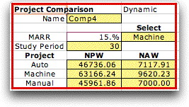
More
than two projects can also be compared by first defining
the projects and then choosing Compare Multiple from
the Economics menu. The figure below shows the form
for the comparison of three mutually exclusive alternatives.
The details of the example are provided in the Computations section.

|
| |
The add-in automatically
determines the study period as the least common multiple
of the lives of the alternatives. The NPW and NAW measures
are displayed on the form and the best alternative is selected.
Incremental analysis can be performed for more than two
projects by ranking the alternatives in order of initial
investment. The alternatives are considered in a pairwise
fashion until the best is determined. The add-in does not
perform this analysis automatically, but the user can do
the appropriate steps by a formulating a series of pairwise
comparisons. |


