| The Economics add-in
can be used to evaluate a single project using time-value
of money principles. The evaluation assumes that all investments,
revenues and expenses associated with the project over
its entire life are known with certainty. The purpose of
the evaluation is to show whether the project meets a specified
criterion for acceptability. The usual criterion for acceptance
is the minimum acceptable rate of return for the investor.
This page shows a summary of the steps of the evaluation.
More detail is available on the pages describing the Economics add-in. |
The Problem
|
| |
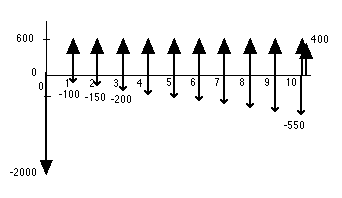
A businessman
is considering the purchase of an asset that has an initial
cost of $2000. The asset promises an annual return of
$600. It's operating cost is $100 the first year, $150
the second, and increases by $50 in each subsequent year.
The salvage value for the asset in 10 years is $400,
or 20% if its initial cost. The cash flow for this situation
showing the individual components explicitly is in the
figure below. If the businessman's minimal acceptable
rate of return is 10%, should he invest in this project?
|
The Project
|
 |
|
Install the Economics add-in.
Choose Add Project from the menu.
Fill in the dialog with the number
of cash flows (3, one for the revenue, one for the
uniform part of the operating cost, and one for the
gradient part of the operating cost). Fill in the number
of investments (1 for the 2000 investment at time 0).
Fill in the Minimum Acceptable Rate of Return (MARR
= 10%) and Life (10 years). These can be changed later.
The bottom half of the dialog is used when taxes and/or
inflation is to be modeled.
|
| |
|
 |
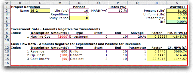
The add-in creates a form
with some items filled in. Specify the investment in
row 9 as a negative number. The Salvage is
the percentage of the investment that is returned at
the end of the life of the asset (20% = 400/2000). The Start value
indicates when the asset is put into service and the End
value indicates the end of its life.
The return is entered in row 13 as a uniform series
with value 600. The first payment time (at the end of
year 1) is entered in the Start cell and the
last payment time (at the end of year 10) is entered
in the
End cell. The uniform part of the operating
cost is entered in row 14 as a negative number (-100).
The operating cost is increasing by an amount $50 per
year. This is entered as a negative gradient (-50) in
row 15. The Start cell indicates when the first
non-zero payment occurs (2) and the End cell
indicates when the last payment occurs. The Parameter for
the gradient is the periodicity of the payments (1 means
that it occurs annually). All the words and numbers
in the white cells can be changed. |
The Results
|
| |
The yellow
cells in column S are computed by formulas inserted
by the add-in. These are the results of the analysis.
Cell S9 is the present worth of the investment considering
both the amount of the investment and the salvage. Cells
S13 through S15 hold the present worths of the annual
cash flow components.
Cell S2 holds the sum of the investment and cash flow
present worths. The is the net present worth of the
project over its life. Since the value (81.93) is positive,
the investment returns more than 10%, the MARR. This
implies that the investment should be acceptable to
the decision maker. A negative value implies that the
project does not return the MARR. Cell S3 holds the
equivalent net annual worth of the project. It is also
positive because it is proportional to the net present
worth. Cell S4 holds the present worth over the study
period. Since the study period (10) is the same as the
life, this is the same as the present value over the
life. |
The Internal Rate of Return (IRR) |
| |
 |
The internal rate of return
is the interest rate that makes the net present worth
of the project equal to zero. It is a measure of the profitability
of the project. It is discovered by a binary search procedure.
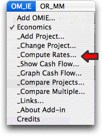
Selecting Compute Rates presents the dialog below.
The project E6_2 is selected from the Name field.
For some projects there may be more than one solution
that yields a zero net present worth. Different solutions
may be found by specifying the initial guess and range
of the search process. The example is called a simple
investment since a single investment is followed by net
revenues in the following years. This kind of investment
has only one solution for the IRR. |
|
| |
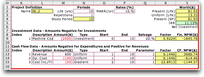
The add-in successively
changes the MARR in cell P1 until the IRR is determined.
The rate is placed in cell S5 on the project definition.
It is colored green to indicate that the number is computed
by an algorithm. If some of the parameters of the project
are changed, the yellow cells will automatically compute
new values. The IRR cell will not change, however, unless
the algorithm is run again.
The IRR is 11.13% for the example. The fact that it is
greater than 10%, the MARR means that the project is acceptable.
The IRR will always be greater than the MARR when the
project net present worth is positive. |
The Cash Flow |
| |
|
For a complicated project
with several cash flow components, it is often difficult
to determine the flow of cash values in the several years
of the project life. For a tabular presentation choose
Show Cash Flow from the menu. In the resulting
dialog, choose the project in the name field. The buttons
on the right select the results to be displayed.
|
|
| |
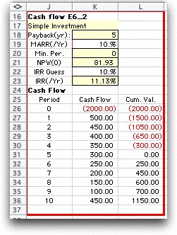
We have chosen to
display the cash flow in each period and the cumulative
values. At the top of the display is a series of measures
that are computed with the Excel economic functions. Row
17 indicates that this is a simple investment, implying
that the cumulative cash flow has only one zero crossing.
In this event the IRR is unique. The Payback is
the number of periods before the initial investment is recovered.
The MARR is an input value. Row 20 holds the minimum period
index, necessary for some of the computations. The NPW(0)
is the net present worth at time zero. The IRR guess is
an input that will effect the computed value of the IRR
if that value is not unique. Row 23 shows the computed value
of the IRR. |
Graph of the Cash Flow
|
| |
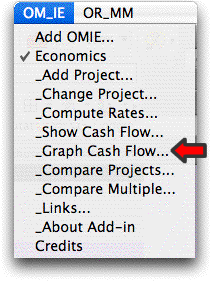 |
It is often instructive to
view a graph of the cash flow. Select Graph Cash Flow
from the menu and select the project name in the
dialog. The terms Actual and Real refer
to different evaluations of the dollar amounts when inflation
is considered. With no inflation, we use Actual to
refer to the cash amounts at each period. The Cash Scale
and Time Scale control the size of the display.
A cash flow table must have already been constructed
for a project to appear on the name list. |
|
| |
The cash flow for
the example is graphed below. Cash amounts at the same time
are accumulated to a single value. For example the 450 appearing
at time 10 is the sum of the salvage value of 400 and the
net income of 50. |
|
| |
We have illustrated
the evaluation of a single project when inflation and
taxes are neglected. The form holding the project data
may be much more complex than the simple example presented
here. A project may have several investments occurring
at different times and many annual receipts and disbursements.
There is no limit to the complexity the add-in can handle
except the size of the worksheet and the limitations of
the user's computer.
The evaluation of projects with taxes and inflation is
more complex requiring additional data and more difficult
computations. The add-in handles these variations using
commands and dialog boxes similar to those illustrated
on this page. |


