A type of problem most often identified with
the linear program is the problem of distributing scarce resources
among alternative activities. In this example the scarce resources
are times available on four machines and the alternative activities
are the production volumes of five products. The machine requirements
in hours per unit are shown for each product in the table
below. With the exception of product 4, that does not require
machine 1, each unit of product must pass through all four
machines. The unit profits for each product are also shown
in the table. There are four machines of type 1, five of type
2, three of type 3 and seven of type 4. Each machine operates
40 hours per week. The linear programming model is to determine
the optimum weekly production quantities for the products.
The goal is to maximize total profit.

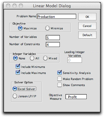
To enter the model for this situation, select
the Linear/Integer item from the OR_MM menu. The dialog defining
the structure of the linear model is presented. Fields are
available to define the Name, number of variables and number
of constraints for the model. Buttons determine whether the
problem is a maximization or a minimization, and the integer
character of the variables of the problem. The variables may
be specified as no integer, all integer, or mixed. In the
latter case the field to the right of the buttons determines
the number of leading integer variables. For a mixed problem,
the leading integer variables have the smallest indices. Additional
integer variables may be specified by placing the letter I
before their indices on the model worksheet.

One important point concerns the Problem
Name. The entry here is used to provide Excel names
to many ranges on the worksheet. The name must satisfy
Excel's restrictions for naming ranges, that is: the
names must not contain spaces, they must start with a
letter and they may not include punctuation marks. If
an error occurs when this dialog closes, try a different
name for the problem. The program automatically suggests
names like LP_1, LP_2 and so on. The user may prefer
a more descriptive name.
The fields below the integer definitions determine
some features of the model that will affect the data entry.
When the Include Minimums box is checked, a row is
provided to hold values for the minimums of the decision
variables. If no row is provided, each variable is restricted
from below by 0. When the Include Maximums box is
checked, a row is provided to hold values for the maximum
values or upper bounds of the decision variables. If no
row is provided, the upper bounds are assumed to be infinitely
large.
The Sensitivity Analysis checkbox determines
whether the solution procedure will create a sensitivity analysis
worksheet after performing the optimization. With the Random
Problem option selected, the program generates data for
the model using random numbers. Otherwise, all data items
will be 0, except the constraint bounds, which will be given
large values. The Show Comments checkbox will install
Excel comments on important cells of the worksheet. This helps
to understand the purpose of the various cells and ranges.
The objective measure field specifies the measure
to be maximized or minimized. Here we are maximizing the
profit.
The Solver option specifies the solution
add-in to be used. Either choose the Excel Solver or
the Jensen LP/IP Solver add-in. When
using the Excel
Solver it
is important that the Solver dialog be opened before trying
to construct a model. Then the model is automatically loaded
into the Excel Solver when the model structure is placed
on the worksheet.
Most of the options on the original model dialog
can be changed by using the Change button that is placed
on the model worksheet.


