|
|
 |
Continuous
Distributions |
 |
-
Beta |
 |

|
The Beta distribution
is important because it has a finite range, from 0 to 1, making
it useful for modeling phenomena
that cannot be above or below given values. The distribution
has two parameters,  and and
 ,
that determine its shape. When ,
that determine its shape. When  and and  are
equal, the distribution is symmetric. Increasing
the values of the parameters decreases the variance. The symmetric
case is illustrated in the figure below. are
equal, the distribution is symmetric. Increasing
the values of the parameters decreases the variance. The symmetric
case is illustrated in the figure below.
The Uniform distribution is the special case of the Beta distribution
with  and and  both
equal to 1. both
equal to 1. |
| |
|
| |
When  is
less than is
less than
 the
distribution is skewed to the right as shown below. When the
distribution is skewed to the right as shown below. When  is
greater than is
greater than  the
distribution is skewed to the left. When the
distribution is skewed to the left. When  =
1 and =
1 and  =
2, the Beta distribution is a triangular distribution with
the mode at 0. =
2, the Beta distribution is a triangular distribution with
the mode at 0. |
| |
|
Generalized Beta |
 |

|
A linear transformation of a Beta
random variable provides a random variable with an arbitrary
range. The distribution is often
used when an expert provides a lower bound, a, upper
bound,
b, and most likely value, m, for the time
to accomplish a task. A transformed Beta variable could be
used to represent
the time to complete a task in a project. The transformed distribution
is called, the Generalized Beta. It's mean, variance and
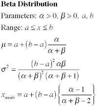
mode are shown at the left.
|
 |
Example


|
Example:
Consider the following hypothetical situation. Historical
grades in a senior engineering class indicate that on average
27%
of
the
students received an A. There is variation among classes, however,
and the proportion must be considered a random variable. From
past data we have measured a standard deviation of 15%. The
current class has 50% A grades. What is the probability that
a proportion of 50% or higher would be obtained from the population
of all exams?
We model the proportion of A grades with a Beta
distribution because proportions naturally fall within the
range [0,1].
The data estimates the mean proportion as
0.27. The standard deviation is specified as 0.15 (variance
0.0225).
We use this data to estimate  and and
 .
We solve for .
We solve for  as
a function of as
a function of  and and
 . Substituting . Substituting
 =
0.27 into this expression, we obtain =
0.27 into this expression, we obtain  =
2.7037 =
2.7037 . .
|
| |
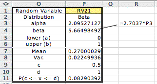
To solve this problem
we created the Beta model as shown at the ABOVE. We use a mathematical
expression in the cell for  .
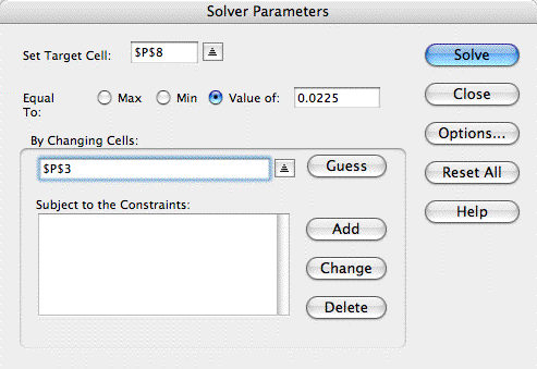
We then use the Excel Solver to find the value of .
We then use the Excel Solver to find the value of  that
results in a variance of 0.0225. The form shows the results
of the Solver analysis. The probability that the proportion
is 50% or higher is about 8%. The current class is exceptional. that
results in a variance of 0.0225. The form shows the results
of the Solver analysis. The probability that the proportion
is 50% or higher is about 8%. The current class is exceptional.

|
| |
|
|


