|
|
 |
Random
Variables |
 |
Discrete Distributions
|
| |
A discrete
probability distribution function is completely described by
the set of possible values the random variable can take and by
the probabilities assigned to each value. On this page we describe
the general features of discrete distributions. On the following
pages we describe a variety of named distributions. All are available
from the Random Variables add-in. We use the triangular
distribution pictured below for an example. |
 |
|
| |
|
The mathematical notation
for a discrete distribution is shown at the left. The values
associated with
a distribution are often integer, but in general they need
not be. For a discrete distribution, only the values in the
set X have
nonzero probabilities and these must be nonnegative. For a
valid distribution, summing
the probabilities over the set X must yield
the value 1.
The number of values in X may be finite or
infinite. When the number is infinite, the set must be countable
infinite. An example is the set of all nonnegative integers.
When the possible values are integers, we will often use k rather
than x as the notation for the values. We use PDF
to refer to the Probability Distribution Function. |
| |
The example experiment
involves throwing a pair of standard dice. Each die has the numbers
{1,2,3,4,5,6},
so the sum of the two dice ranges from 2 through 12. The value
with the greatest probability is called the mode, so
7 is the mode of this distribution. The probabilities
sum to
1
and all
probabilities are nonnegative, so this is a valid distribution. |
| |
|
| |
|
The Random Variables add-in
defines distributions using named ranges on the worksheet. For
the example, the range B2:B5 has the name Dice. The Mean and Variance in
B6 and B7, as well as the probabilities in B9 through B19, are
computed with user-defined functions provided by the
add-in. |
| |
|
|
Moments |
| |
|
Several quantities can be computed
from the PDF that describe simple characteristics of the distribution.
These are called moments. The most common is the mean, the
first moment about the origin, and the variance, the second
moment
about the mean. The mean is a measure of the centrality of the
distribution and the variance is a measure of the spread of
the distribution about the mean.
The skewness is computed from the third moment about
the mean. This quantity can be positive or negative. We normalize
the measure by squaring the third moment and dividing it by
the third power of the variance. To recover the sign
of the third moment, we multiply this ratio by the sign of
the third moment. The skewness indicates whether the distribution
has a long tail to the right of the mean (positive) or to the
left (negative). The skewness is 0 for a symmetric distribution.
The kurtosis is a measure of the thickness of the
tails of the distribution. The use of this measure is not obvious
in most cases, but it is included for completeness. The formula
for this measure subtracts 3 from the ratio of the fourth
moment about the mean and the square of the variance. The Normal
distribution has a kurtosis of 3, so this normalization provides
a value relative to the value for the Normal
distribution. It can be positive (greater than the Normal)
or negative (less than the Normal). |
| |
|
The moments for the dice example
are computed with user-defined functions functions
provided by the add-in. |
| |

|
We use distributions to answer questions about situations that
involve random variables. We use the game of Craps to illustrate
the use of the triangular distribution. In this game, the player
roles a pair of dice. We assume the player is
female. If on the first roll of the dice the player throws a
7 or 11,
she
wins.
If the
player
throws
2, 3 or
12, she loses. If the player throws
a number
other
than 2, 3, 7, 11, or 12, the number thrown is called the
point. If the player does not win or lose on the first roll,
she must roll the dice again and continue to roll
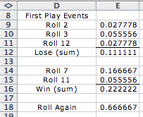
until she throws the point and wins, or a 7, and loses. The triangular
distribution describes a single roll of the dice. Since the alternatives
are mutually exclusive, probabilities of an event involving
several different results are obtained by summing. We compute
the probabilities associated with the first throw at the left.
We use the Craps game as an example for several other distributions
on the following pages. |
Named Distributions |
| |
It is useful for modeling
purposes to know about the named discrete distributions. When
an experiment on which a random variable is based satisfies the
logical conditions associated with a named distribution, the
probability values for the random variable are immediately determined.
Then we can use the distribution without extensive experimentation
to answer decision questions about the situation. We consider a
number of named distributions on the following pages. Click on
a link at the far left for descriptions and examples. |
| |
|
|


