 |
|
An interior point demonstration is included
in the add-in collection as part of the Teach LP add-in. Access
to the demonstration is via the menu item at the left. The
dialog defining the model is the same as that used for the
tableau and revised simplex options, except we allow only
Demonstration and Run solution options. The Demonstration
option shows each step of the process while the Run option
completes all steps without interruption and presents a summary
of the solutions.
The examples for this section are in the Teach
LP demo (teachlpdem.xls). To solve or change the model you
must have the Teach LP add-in loaded. Use the Relink buttons
command to establish links to the worksheet buttons.
|
| |
All forms of the simplex
method reach the optimum by traversing a series of basic solutions. Since
each basic solution represents an extreme point of the feasible
region, the path followed by the algorithm moves around the
boundary of the feasible region. In the worst case, it
may be necessary to examine most if not all of the extreme
points. This can be inefficient since
the number of extreme points can become very large.
In
contrast to the simplex algorithm, interior point methods approach
the optimum from the interior of the feasible solution space.
Only in the limit does the solution approach an optimum
solution at the boundary of the feasible region. The development
of the interior point methods is a very important step in the
theory and practice of optimization. Such methods are available
in most optimization packages. We cannot describe the mathematics
of the method in this discussion. Refer to Chapter 4 of the
ORMM text for a complete discussion of the background of this
add-in and several excellent references. This add-in implements
a path finding algorithm known as the primal-dual
path following algorithm which has become the method
of choice in large scale implementations.
In developing the algorithm, we will work with the primal
and dual problems as defined below. The primal problem
is assumed to consist of m nonredundant equations
in n variables, and is given in equality form. This
means that the n dual variables, π,
are unrestricted in sign. The m-dimensional
vector of nonnegative slack variables, z,
transforms the dual inequalities to equations.

|
| |
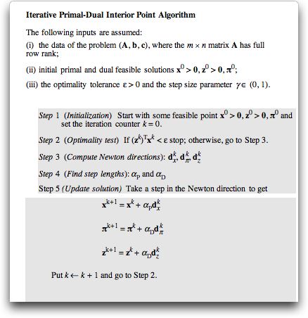
The algorithm starts
at some solution and takes a series of steps toward the optimum.
The process stops when a gap measuring the difference between
the primal and dual objective values reaches a present limit.
A brief survey of the path-finding algorithm is below.
|
| |
We apply the method
to a small example below. The primal and dual problems can
be represented with two structural variables so it is possible
to graph the paths taken in the search for the optimum. This
are shown below. For the primal problem the feasible region
is between the sloping lines and the axes of the graph. For
the dual problem the feasible region is above the sloping lines.
The figures clearly show how the paths traverse the interiors
of the feasible regions. |
|
Small Example |
| |
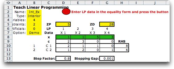
The small example
is shown below. The step factor indicates that the
|
| |
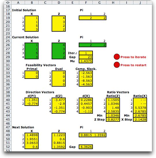
The add-in constructs
a form that calculates all relevant quantities for the add-in.
The initial form is below. The green regions, X, Z and Pi,
are maintained by the program. The yellow regions all contain
formulas to compute the necessary vectors. The solution moves
in a direction described by the vectors starting in row 38.
The step size is determined by finding the largest step that
will move to a boundary. That step is multiplied by the Step
Factor to assure that the method never actually goes to
a boundary of the feasible region.
|
| |
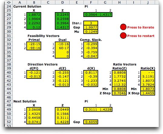
Clicking the Iterate button
takes the step from the initial solution to the first solution.
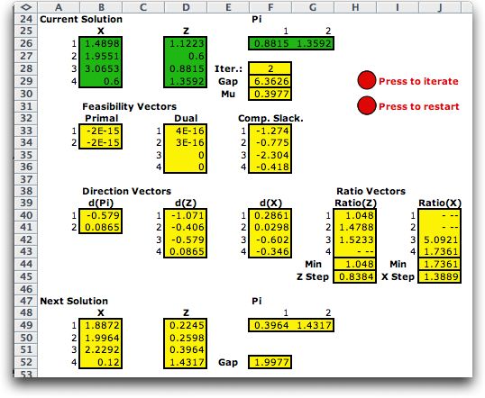
The next step is below.
|
| |
Notice each step computes
both the primal and dual solutions and the gap becomes smaller.
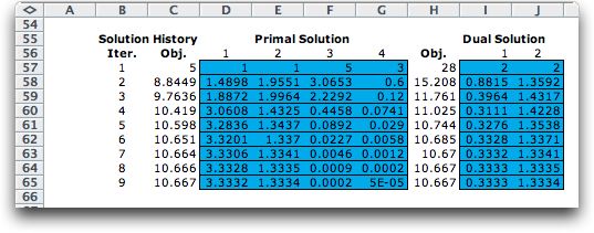
When the gap falls below 0.001, the process stops and the program
presents a history of solutions.
|
Larger Example |
| |
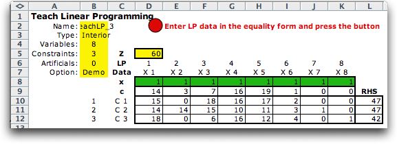
Here
we use
the same example used earlier to compare the results with those
obtained by the simplex method. The figure below shows the
example problem. In the case of the interior point method,
no artificial variables are added. We have chosen the initial
solution as all 1's.
Clicking the button causes the algorithm to look
for a feasible interior solution. In this case, it was not
successful and generates the following dialog.

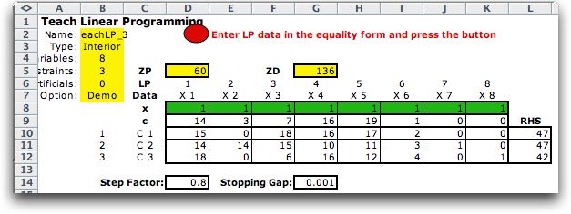
The model after the initial step is shown below.
The interior point method works with the primal and dual solutions.
There values are shown as ZP and ZD in the figure.
|
| |
Data cells are provided for the Step factor and
the Stopping Gap. The Step Factor determines how close a step
will come to the boundary of the feasible region. A step of
1 goes exactly to the boundary. A number less than 1 should
be entered. The Stopping Gap holds the minimum value of the
primal dual gap. The program stops when the gap reaches this
level. The student controls these values by entering numbers
in the cells. They may be changed during a demonstration run.
The following discussion describes the several
arrays that are placed on the Excel worksheet. Yellow areas
contain formulas that implement the interior point method. |
| |
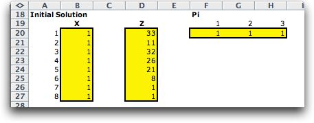
Initial
Solution
A simple algorithm attempts
to find interior solutions for the primal and dual problems.
The algorithm will not work unless the last m columns
of the primal constraints form a nonsingular matrix. If the algorithm
is successful the initial values of x, z and pi are
set to the interior values; otherwise they are all set to 1.
The interior point algorithm is usually successful with a non-interior
start, but it may fail. In the case of the example, the program
did not find an interior primal solution and the primal variables
are set to 1. With a non-interior initial solution the gap measure
is changed as described below.
|
| |
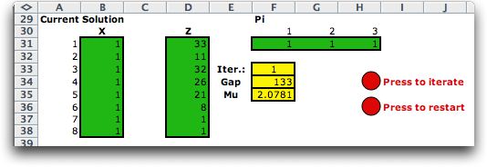
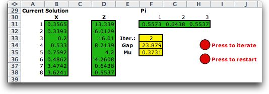
Current Solution
In the first iteration the initial solution is
placed in the arrays holding the current solution. Note that
these arrays are colored green indicating that they do not
hold formulas, but are manipulated by the algorithm in the
add-in. Also shown on the figure is the iteration number, the
gap measure and the value of Mu. When the initial solution
is interior we use the difference between the dual and primal
objective values as a gap measure. This gap is always positive
for interior solutions and decreases as the iterations progress.
If the solutions are not interior, the gap as
defined above may become negative and is no longer a good measure
of optimality. In this case, the program changes the gap to
the product of the x and z vectors. Because the
optimal solution will satisfy primal-dual complementary slackness,
this measure should approach zero as the solution approaches
the optimum. Note that it is important that both x and z be
strictly positive.
|
| |
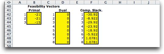
Feasibility
and Complementary Slackness
The primal and dual feasibility
vectors tell whether the corresponding solution is feasible.
The vectors are 0 for feasible solutions. For the first iteration,
the vectors show that the primal solution is not feasible, while
the dual solution is feasible. The vector labeled Comp. Slack.
is a measure of complementary slackness. It should approach 0
as the iterations progress.
|
| |
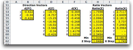
Direction
and Ratio Vectors
The direction vectors
show directions in which pi, z and x should
change to move toward feasibility and optimality. The ratio vectors
tell how far each component can change to remain interior to
the region. The smallest ratio indicates the maximum change that
will move to a boundary. We multiply that step by the step factor,
less than 1, to determine how far to move.
|
| |
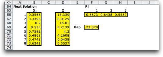
Next
Solution
The next solution is
reached from the current solution by taking the indicated step.
|
| |
Taking
the next step
The iterative process
continues by moving the next solution to the arrays for the current
solution. The formulas on the sheet calculate the new next solution
and the process continues. The procedure terminates when the
gap reaches the specified smallest value.
|
| |
The
History
The program keeps a history of the primal (x) and dual
(pi) solutions as the algorithm progresses. The history
for the example is shown below. |
|
| |
Final Solution
The final solution is shown in row 6 of the
model. All variables are strictly positive as required by an
interior solution, but X1, X3, X4, X6 and X7 are very small.
If you refer to the solutions obtained by the simplex method
you will find that these are the nonbasic variables at optimality.
For an extreme point these all all zero. The corresponding
values of the basic variables are: X2 = 1.185, X5 = 2.765,
and X8 = 8.824. The interior point method approaches the extreme
point, but never reaches it. In some cases where an extreme
point solution is required, additional processing of the solution
is necessary. There are methods for finding extreme point solutions,
but none are included in the add-in.

|
| |
This add-in was not meant
to be a solution of a large linear programming model, but it
succeeds very well at illustrating the concepts and providing
small numerical examples. |
| |
|


