 |
|
The revised primal simplex method uses matrix
operations to compute the quantities used by the simplex
method. We have implemented this technique with an Excel
add-in called Teach LP. This unit is the introduction to
that portion of the add-in that performs the revised simplex
method. To run an exercise first load the Teach LP add-in
and then select Revised
Simplex from
the menu.
The dialog defining the model is the same as
that used for the Tableau simplex method and specifies the
number of variables and constraints in the equality form
of the LP model.
|
| |
The revised simplex
method performs the same steps as the tableau method but does
not keep the tableau as an aid. Rather, whenever the
algorithm requires a number from the tableau it is computed
from one of several matrix equations, often involving the inverse
of the basis. The data for the algorithm are the matrices A, c and b defining
the original problem, the number of variables and constraints, n and m,
and a record of the current basic and nonbasic variables. The
basis matrix, B, that is a square matrix
composed of the columns from A corresponding to
the basic variables.
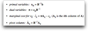
The components of the revised simplex algorithm require the
computation of following information:

The add-in constructs a worksheet that automatically
calculates these formulas. By clicking buttons
placed on the worksheet, the student or teacher can go through
the steps of the primal simplex. |
Example |
| |
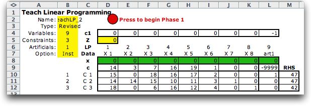
The randomly generated
model used as an illustration for this section is shown below.
The model has been modified by including an artificial variable
for the first constraint. The details of this modification can
be found in the tableau method page.

|
Initial Basis |
| |
Pressing the Phase
1 button, initiates the process that builds the vectors and
matrices that implement the simplex procedure. The figure below
shows the initial basis and basis inverse matrices. These are
placed to the right of the LP model. The matrices change during
the algorithm as the basic variables change. The matrices are
colored yellow to indicate that every cell contains a formula.
Yellow entries should not be modified by the user.

|
Revised Simplex Matrices |
| |
The other information
necessary for accomplishing the revised simplex procedure is
placed in the rows below the LP model as shown below. As for
the tableau method, the Iterate button initiates the iteration,
first asking for the variable to enter the basis, then the variable
to leave the basis. Starting in row 20, the cells are colored yellow
indicating that they contain Excel formulas that compute
the quantities necessary for the iteration. The basic variable
indices in row 19 can be changed to experiment with different
bases, however the add-in will control these entries as well
as the entering and leaving variables. |
|
Selecting the Entering and Leaving Variables |
| |
With the Instruction option
for interaction, the program presents a dialog for selecting
the entering variable. The student should enter the index of the
entering variable. On the first push of the Hint button,
the negative reduced cost entries are colored. The second hint
automatically enters the index of the variable with
the most negative reduced cost. Clicking OK selects X3 to enter
the basis. |
|
| |
Then the student is asked
to select the leaving variable. The hint button colors first
the entering column and then the cell with the minimum ratio
column. The third hint automatically places the index of the
leaving variable into the cell. |
|
| |
Finally, the student
must click the pivot button to change the basis. |
|
| |
Pressing the Pivot key
replaces index 9 in the vector of basic variables (the artificial
variable) with the index 3. Since all the cell contents are
controlled by equations, the cells all change to represent
the new basis. For the example, the objective value of 0 indicates
the end of phase 1. Clicking the button will begin phase 2. |
|
Phase 2 |
| |
The Phase 2 button
replaces the Phase 1 objective with the Phase 2 objective in
the formulas for the values of the dual variables and reduced
costs. |
|
| |
Most of the formulas
on the revised-simplex display are governed by the basis inverse.
The basis is automatically maintained in the columns Q through
S. The columns of the basis are selected from the constraint
matrix by the indices in row 6. We see in Q7...S7 the values
of the objective coefficients for the basic variables. The
range W8...S11 holds the basis constructed by the indices
in Q6...S6. The range Q8...Y11 holds the inverse of the basis
computed with the Excel INVERSE function. The range W8...Y8
holds the dual variables.

|
| |
The procedure continues
in Phase 2 with the 5th variable replacing the 3rd variable in
the basis. |
|
The Optimum Solution |
| |
One more step leads to
the optimum solution. |
|
| |
The
final solution appears in the x-vector of the original LP model. |
|
| |
The basis, inverse
basis and dual variables. at optimality are shown to the right
of the LP model display.

|
| |
We have illustrated the Instruction solution
option that displays each iteration and allows student interaction
in selecting the entering and leaving variables. The Demonstration option
presents the same results with the computer making automatic
decisions. The Do it Yourself option, does not provide
hints. The student can make arbitrary basis change decisions. |
| |
|


