The capital budgeting problem will be solved with integer programming. To create a model, the Math Programming add-in must be installed. The model may be solved with either the Jensen LP/IP Solver or the Excel Solver. In the case of the Jensen Solver the LP/IP Solver add-in must be installed. There is no need to create a model, as the add-in automatically constructs the required model.

If the Excel Solver is used, that add-in must be installed. When it is installed, the command "Solve..." will appear on the Tools menu. Be sure to open and close the Excel Solver dialog before attempting to create or solve a model. This will establish a connection to the add-in.

The optimum portfolio for the example is shown below. For a budget of 650, the portfolio consists of projects 1, 2, 4, 5, 6, and 9. The portfolio has a NPW of 266 with an investment of 650. The internal rate of return for the portfolio is 18%.

The optimum solution for any budget can be obtained by changing the budget cell and selecting the Solve button from the Actions dialog.

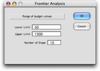
We discover the efficient frontier by varying the budget and finding the optimum solutions for each of several budget levels. To find the efficient frontier choose the Frontier action from the Choose Action dialog. A dialog then asks for the range of budget values for the frontier. The minimum value is the minimum investment and the maximum is the sum of the investment values for projects that have positive NPW values. These numbers may be changed by the analyst. The range between the lower and upper limits is divided into the number of steps specified in the dialog.

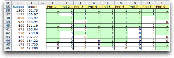
For each step in the range, the solver finds the optimum solution and presents it in the list of frontier solutions. The green fields indicate the projects selected at each level.

A graph of the frontier is constructed below the solution list. A characteristic of the solution frontier is that no feasible solution determines a point (budget, return) above and the to left of frontier. All feasible solution points lie below and to the right of the frontier. Because of the discrete nature of the solution variables the curve is not concave, but it must be monotonically increasing.

The Math Program action on the Choose Action dialog reveals or hides the rows holding the math programming model. When the model is initially constructed the rows hidden. Selecting this action unhides these rows. The figure below shows the model for the example problem. Yellow cells hold formulas, so they should not be changed. For the illustration the second constraint has no effect.

The capital budgeting problems in this section are all modeled as mathematical programming models. These models can be controlled directly through the Math Programming add-in. To create control buttons, choose the Relink Buttons command on the Math Programming menu. New control buttons are added as in the figure below. The Change button can be used to add and subtract variables and constraints. Before adding constraints, however, be sure to insert rows before the project definition table or the new rows in the math programming model will overwrite parts of the table. Integer programming models will accept a variety of logical restrictions as long as they can be described with linear expressions. The Change button also allows the Solver to be changed.