The multiperiod option creates a model similar to the capital budgeting problem but explicitly represents the individual time periods during the time horizon. Projects with non-uniform cash flows are easily represented on the data form. The most useful new feature is that cash flow demands can be specified for the individual periods and feasible portfolios must generate sufficient cash flows to provide for these requirements. To create a model choose Multiperiod from the Portfolio menu. We use an example adapted from class notes by A. Ruszczynski.

Three bonds are available to the investor. The cash flows for one unit of each bond are shown below. The negative number for year 0 is the initial investment and the positive numbers for the remainder of the years are the returns from the bond. Note that all bonds have no return in your 1. All cash flows occur at the end of the year. Investment\Year 0 1 2 3 4 5 6 7 8 9 10 11 12 13 14 15 Bond 1 -980 0 60 60 60 60 1060 Bond 2 -970 0 65 65 65 65 65 65 65 65 65 65 1060 Bond 3 -1050 0 75 75 75 75 75 75 75 75 75 75 75 75 75 1075 Multiple units of each bond may be purchased from an investment budget of $250,000. Fractional amounts may be purchased. The portfolio must yield cash flows in the fifteen years as shown in the table below. The amounts are in $1000's. Cash is distributed at the end of each year. Year 1 2 3 4 5 6 7 8 9 10 11 12 13 14 15 Requirements 11 12 14 15 16 18 20 21 22 24 25 30 31 31 31 The investor is to select the number of units for each bond to meet the cash requirements and maximize the total cash available at the end of the last year (year 15). Cash not invested in the bonds earns a 5% return.

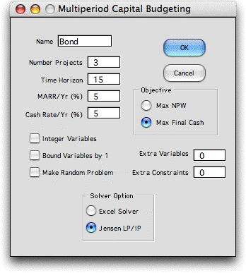
The Multiperiod menu item calls the dialog shown below. The number of projects is 3 to represent the three bond alternatives. The time horizon is 15. Excel financial functions used on the worksheet limit the time horizon to 28. We choose to maximize the final cash flow.

In addition to the MARR entry that is used to calculate net present worth values, we must include a rate for cash either not used by the initial investment or cash generated by the investments but not used immediately for cash requirements. We choose 5% for both quantities.

The Integer Variables checkbox and the Bound Variables by 1 checkbox are left unchecked for this example.

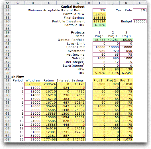
On clicking OK, the program builds a form to hold the data for the problem and calls the Math Programming add-in to construct a model. The form for the data describing the projects is placed below the math programming model. The model is hidden by hiding the worksheet holding the model. The form the example is shown below. Although the returns for the example are not entirely uniform because of the zero returns for year 1, it is convenient to enter the data for the three parameter cash flow (investment, return and salvage) in the range I44 through K47. The data for the cash flows is in the range (I53 to K68). Most of these entries are formulas transferring the data defining the projects to the individual cash flow amounts, however, we have replaced the formulas with 0s for period 1. The NPW and IRR values in rows 48 and 49 are computed from the period data starting in row 53.

The solution shown in the figure above is shown in the green cells of row 41. Initially all variables are zero, indicating no bonds are purchased and the entire budget is saved. Interest from the savings is in column F and the current balance is in column G. Column E shows the returns from the bond investments. These values are 0 since the initial solution purchases no bonds. The requirements are in column D. The final savings after all withdrawals is 88,487. It is this number that we will try to maximize.

Generally we indicate cells that hold formulas with yellow backgrounds and cells that can be changed with white backgrounds. For this application however, the cells holding the project cash flows can be changed as required by the situation.

The figure below shows the form after the Solve action has been chosen. The solution in this case was obtained with the Jensen LP/IP add-in. Cells I41 to K41 show the optimal portfolio. The savings play a significant role in satisfying the withdrawals.

When we construct a second model with the goal of maximizing the NPW of the portfolio the solution is the same as the one above. When the MARR is the same as the rate of return on savings, maximizing NPW is equivalent to maximizing the final savings.

Part of the math programming model is shown below after the solution has been obtained. The model is linear and continuous, so its solution an be obtained with linear programming. The data for the problem is automatically placed on the math programming model, so there is no need for the analyst to interact with the model unless extra constraints or variables have been included.

It is interesting to perform a parametric analysis on the budget to see how it affects the final cash available and the mix between the bonds. We click the Frontier button on the Action dialog. The frontier dialog shows lower and upper limits on the budget. The lower limit is the present worth of the requirements for all the periods not including time 0. The present worth is computed with the cash or savings rate, 5% in this case. This is the amount that must be invested to meet the requirements without using any projects. The upper limit is the sum or the requirements. The limits can be changed. The number of steps is the number of equal ranges between the upper and lower limits. One more than this number will be computed. Only feasible solutions will be displayed.

The solutions computed for the example are below. The solutions have been rounded to the nearest integers.

Because the budget and cash numbers are so large, the program was unable to create a frontier chart. To obtain the chart it would necessary to scale the data so the budget and cash numbers were in the range of 100's rather than 100,000's.

The problem described on this page has an investment constraint plus constraints for each period in the time horizon. Separate variables are used to model the investments chosen and the savings at the end of each period.

The add-in allows several model variations. With the objective to maximize the net present worth of the portfolio and with the variables required to be integer, we obtain a model very similar to the Capital Budgeting problem. For the multiperiod model, however, the period cash flows need not be uniform and specific period cash requirements may be placed on the portfolio. The add-in allows extra variables and constraints to be included in the model. With these a variety of logical constraints can be imposed.

When the maximum NPW is the objective, the objective function of the math programming model will be the weighted sum of the project NPW values. The objective is still linear so linear or linear mixed integer models are appropriate. When the MARR is the same as the interest rate on savings, the two problems are equivalent. When the two rates are different, the two models are not equivalent. When the budget is fixed by some higher level organization that the organization making the capital decisions, the MARR may be set by the higher level organization. Once the budget is received, however, money not spent or recovered from the investments may in fact be kept within the decision making organization, thus justifying the use of a different rate for this money.