|
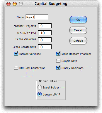
The capital budgeting
model considers risk by computing the statistical variance
(and standard deviation) of each project and selecting the
projects to minimize the portfolio variance. To create a
model that explicitly considers risk, click the Include
Variance box
on the dialog.
|
|
| |
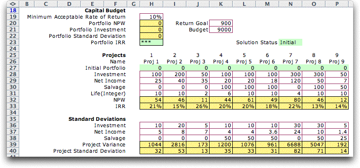
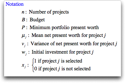
We use
the previous example but assume that the initial investment,
net income, and salvage value of each project are random variables
with specified mean values and standard deviations. For this
analysis the life of a project is not a random variable, but
is fixed. Although it is sometimes convenient to assume Normal distributions
for the random variables, it is not necessary for these results.
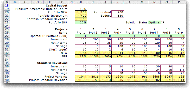
The data for the projects in the example problem are shown
in the table below. We assume that all random
variables are statistically independent.
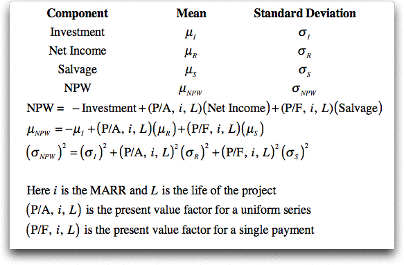
The mean values for the investment, net income and salvage
are given for the example in rows 28 through 30 and the corresponding
standard deviations are given in rows 36 through 38. The project
lives are in row 31. |
|
 |
Using basic definitions
for the mean and variance, it can be shown that the weighted
sum of independent random variables is a random variable whose
mean and variance are calculated as below.
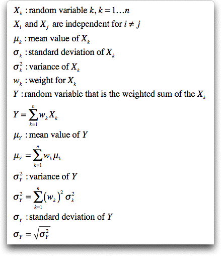
Since the present worth values are computed as
a weighted sum of the components, the mean and variance for
the NPW for each project are computed as below. With the simple
data option, these formulas are not used. Rather the NPW and
standard deviation for each project are entered directly as
data. The variance is the square of the standard deviation.
In the Excel table showing the example earlier
on this page, row
32 holds the values of the mean NPW for each
project, row 39 holds the values of the variance. Row 40 is
the square root of row 39, and holds the standard deviations
of the projects.
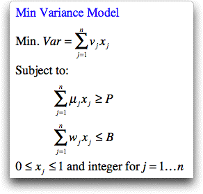
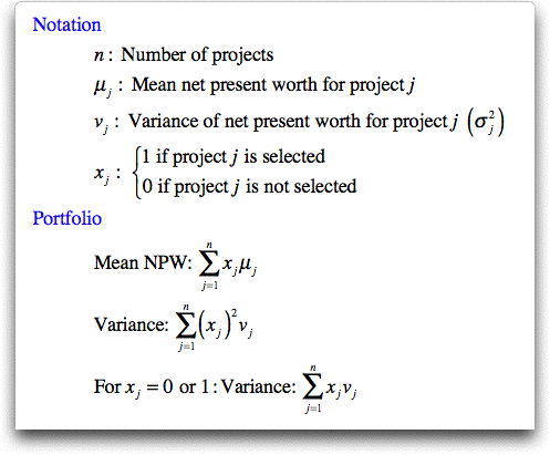
Using the same principles, the mean and variance
of the portfolio can be expressed as functions of the decision
variables. When the variables are constrained to 0 and 1, the variance
is a linear function of the variables. Otherwise, the variance
is a separable quadratic function of the variables.
|
| Math Programming Model |
| |
With these definitions,
several optimization models are possible depending on the goal
of the analyst and the constraints that are included. We choose
to minimize the variance while placing a lower bound constraint
on the NPW. We also include
a budget constraint. The figure below shows the model
when the selection variables are limited to 0 or 1, representing not
select or select. Since the model is linear,
integer-linear programming can be used to find the optimum
portfolio of projects. |
|
| |
The worksheet below
shows the minimum variance solution for the example. Cells
K20 and K21 are provided to hold the return goal (the minimum
NPW) and the Budget respectively. These are controlled by the
analyst. Of course when the cells are changed the model must
be solved to obtain the new solution. The solution below has
the smallest variance when the portfolio goal is to return
at least 200. The budget constraint of 650 is not tight for
this solution since the portfolio investment is only 400. |
|
| |
The math programming model is a linear
program and is in the hidden rows at the top of the worksheet.
The rows may be revealed manually or by using the Math Program button
on the Actions dialog. |
|
| Integer but
not Binary |
| |
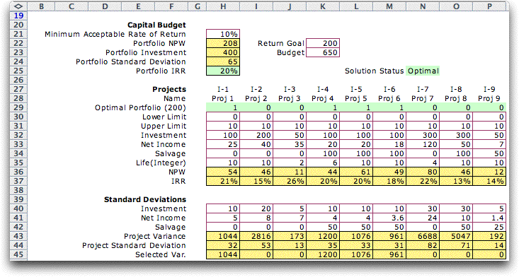
When variables are allowed to
assume values greater than 1 or the integrality restriction
is dropped, the optimization model is nonlinear. Larger values
are allowed if more than one of each project can be purchased.
One might drop integrality when the investments can be made
in fractional amounts.
|
| |
The Excel model for this case
has additional rows for lower and upper limits on the variable
values. The minimum variance solution is shown below when the
return goal is 200. It happens to be the same as the binary
case. |
|
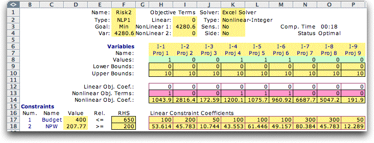
| |
The add-in creates the nonlinear-integer
model below when the variables are not restricted to binary values.
The model has a separable quadratic objective function. Row 13
holds equations that square the variable values. Row 14 holds
the project variances. The model is both nonlinear and integer.
The Excel Solver can solve such models, but the performance is
much reduced in comparison to a linear-integer model. |
|
| Efficient
Frontier |
| |
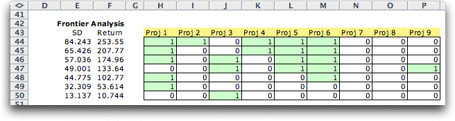
By sequentially solving this problem
with different limits on the NPW constraint, the analyst can
construct a set of solutions each with the minimum variance
for the obtained value of the NPW. We illustrate with the model
having binary variables. We set the budget for the example
problem to be very large and not constraining and solve the
problem for increasing limits on the NPW. A set of solutions
is obtained. Plotting the solutions on a chart with NPW and
variance as the axes, one obtains what is called the efficient
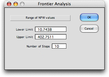
frontier of solutions. To find the efficient frontier
choose the Frontier action. The program
finds the lower limit by setting the NPW constraint limit to
0 and solving the model. The lower limit obtained is the NPW
of the minimum variance portfolio. The upper limit is the sum
of the positive project NPW values. To make a more refined
search, these limits may be changed. The Number of Steps entry
specifies how many individual problems are solved. The NPW
range is divided into this number of equal intervals.
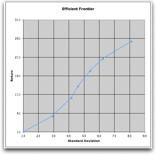
The set of solutions for the example is shown below.
The higher range of NPW values was not obtainable because of
the budget constraint. Portfolios with higher returns have higher
standard deviation values. Each portfolio shown is a minimum
variance portfolio. |
|
| |
The graph prepared by the program
is shown below. This is the efficient frontier. There are no
solutions above and to the left of the frontier line. It is not
concave because of the restriction to integer variables. |
|
| Correlation |
| |
It is conceivable that projects
are not statistically independent. The
returns of dependent projects could be related through a correlation
matrix. Minimizing the variance considering correlation becomes
a non-separable quadratic programming problem. The binary version
has the form of a quadratic assignment problem. Although the
original program included this option, we have deleted it because
of difficulty of solving the problem with the Excel Solver.
Also, it seems unlikely that correlation data would be available
in a practical instance of the capital budgeting problem. |
| |
|