|
|
 |
Estimate |
 |
-
Time Dimension |
 |
It may be desirable to construct a cash flow for the project
that indicates the expenditure of money over time. For an example
we use the WBS with only two levels of detail. This makes the
graphics and data simpler, but similar results can be obtained
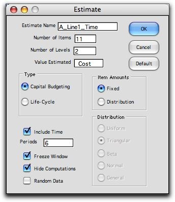
with any level of detail. To add the time dimension, click
the Include Time box as shown below. Also enter the
number of periods of the analysis. For the example we assume
the project will take six months. |
| |

|
| |
In addition to the
WBS, two columns are provided to specify the start and end
time of each activity. |
| |
|
| |
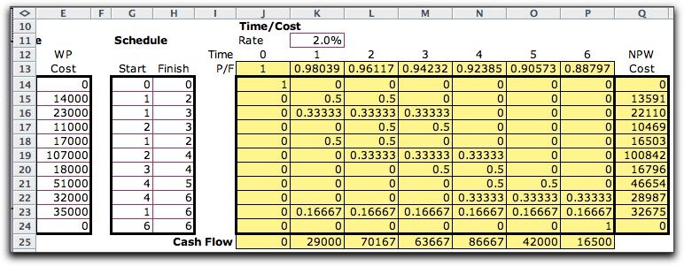
To the right of the
schedule there is a time/cost display showing the six month
period with an additional column for time 0. Column J, for
time 0, holds investment amounts that occur at the beginning
the six month period. There are none for the example. Columns
K through P show how the work package costs are spread over
the six periods. The range is colored yellow to indicate that
it contains formulas. The models assume that the costs are
spread evenly over the intervals defined by the start and finish
columns. These formulas can be manually changed or replaced
by numbers for other distributions of cash flow.
The row at
the bottom of the display, row 25, holds the cash flows for
the six periods. An entry, say K25, is obtained by multiplying
the costs in column E by the proportions in column K. The cash
flows are interesting to the planner concerned with financing
the project. They will also be used for equivalency calculations
in other lessons. |
| |
 |
| |
The numbers in row 13
are the present worth factors, identified by P/F. We will have
much to say about these factors later, but it is sufficient to
say at this point that when a cash flow occurs at some time t,
multiplying it by the P/F factor computes an equivalent value
for the cash flow at time 0 called the net present worth,
NPW. When we multiply a row in our time/cost matrix by the vector
of P/F factors, we obtain the equivalent value
of the entire row of cash flows. We see in column Q the NPW value
for each work package. For positive interest rates, NPW values
are less than the total cash flow. For example, the
cost of 14,000 in row E15 results in a NPW of 13,591. |
Summary |
| |
Clicking the Summarize button at the top of the
page summarizes the total NPW values for the second level activities
and an estimate of the NPW of the entire project. These depend
on the interest entered in cell K11. With an interest rate
of 0, the NPW values are the simple sums of the cash flows
over time. |
| |
|
| |
All the results cells
that are colored yellow hold formulas that recalculate automatically
if any data item is changed. Thus the display is dynamic. |
| |
|
|


