|
|
 |
Estimate |
 |
-
Life-Cycle Costs |
 |
The life-cycle cost, LCC, is the sum of all expenditures
less receipts from origination of the project to disposal of
the system. In additional to the capital costs, the LCC includes
the operating costs and revenues for each year of the life
cycle as well as the disposal cost. When an interest rate is
defined, the LCC is the net present worth rather than the sum.
For this analysis we need a new structural definition,
the cost breakdown structure or CBS. This structure is similar
to the WBS in that it uses a numerical classification system.
Rather than enumerate the activities in a project, however,
this structure enumerates the cost and revenue components of
the life-cycle cost.
There are two problems associated with LCC. The
first is estimating the annual operating cost and revenue.
For systems with some complexity, this is not a small problem
since there are usually a great number of parts associated
with a typical product and a corresponding large number of
individual estimates required. The second problem is estimating
the variation of these costs (and revenues if appropriate)
over time. The life of a typical life cycle may be several
years and the factors that affect cost estimates may well change
over time. Although we use years in this discussion,
any time interval can be used.
The add-in offers two options for cost estimation:
with time and without time. The with time option
estimates the cash flow in each year over the analysis period,
usually the life of the system. The without time option constructs
a form to estimate unit cost as a function of production volume.
We illustrate the without time option on another page. |
Example |
| |
To illustrate,
we consider again the assembly line design project described
in the capital budgeting page. Here we describe the products
that the assembly line will produce once installation is complete.
The line produces three products: A, B and C. The characteristics
of the products are shown in the tables. Manufacturing the
products uses materials and resources. Materials include the
parts and supplies that go into the product. Resources describe
the machines and labor that are used for production. Materials
must be replenished after use. Resources use time and time
is also limited. The materials
and resources are listed by name for the example in the table
on the left.
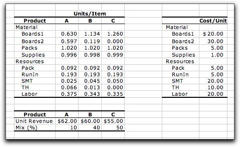
Each product uses different amounts of materials
and resources. These are shown
in the columns labeled units/item. The word
unit refers to a unit of raw material, and the word item refers
to a single finished item. The
table on the right shows the costs per unit for the materials
and resources. The table at the bottom shows the revenue per
finished item for the products as well as the product
mix. The latter is the proportion of the total production devoted
to each product.
The materials and resource units may not be measured
using the same dimensions. For example, resource usage is typically
measured in time dimensions, such as hours, while material
usage is typically measured in quantity dimensions, such as
pounds or part count. For example, the cost for
the first board type is $20 per board, while the cost for labor
is $20/hour. To compute the cost for a component we multiply
units/item by cost/unit and the dimension of the measurement
cancel out. It is important that the dimensions be consistent.
The markets for the products are expected to last
six years. The anticipated annual sales for all three products
are in the table below. We see that production is expected to
grow in the first few years and then decline.

On this page we use this example to estimate
the life-cycle cost of the assembly-line system. We use
the capital cost computed earlier, but assume the disposal or
salvage value of the line is zero. We first analyze a single
product, A, to keep the example small, but then we consider all
three products. |
Add Form |
| |
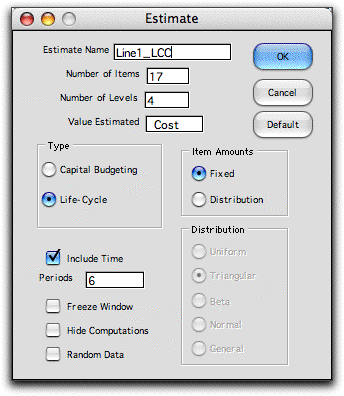
To create a life-cycle
cost worksheet, choose Add Estimate from the menu,
and fill out the dialog as below. With only product A, this
example has 17 items and four levels of detail in the CBS.
Clicking the Life-Cycle button
creates the CBS rather than the WBS. For the example we include
six time periods.
|
| |
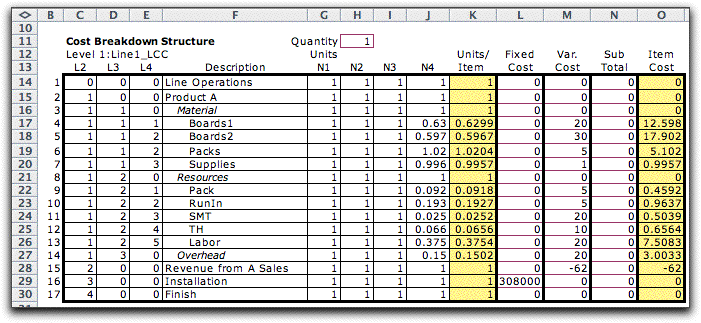
The
data for the CBS is similar to the WBS, except in a few details.
The structure identifies levels of the product structure. The
system is assigned to level 1 with the index 1. We use level
2 for the product definition and to segment between cost and
revenue. Items 3 through 14 are costs, while item 15 is revenue
from sales (entered as a negative cost). Level 3 is used to
divide the cost components into material, resources and overhead.
Level 4 identifies the individual cost elements. Each line
in the CBS is unique with respect to the indices assigned to
the levels. Item 16 holds the installation cost computed on
the capital budgeting page. |
|
| |
The columns
N1 through N4, columns G through H in the worksheet, hold numbers
that compute the total number of units required for each item
of finished good. Usually 1 is used for N1. N2 is the number
of level 2 items used for each level 1 item, N3 is the number
of level 3 items used in the level 2 item, and so on.
For the present case our data specifies the
number of units per item directly and that is entered in column
N4. For example, we see that for each item of product 1, 0.63
Board 1 components are required.
The Units/Item column, column K, holds
the product of the number columns. The number columns are useful
for describing the product structure. We illustrate an interesting
case in the Automobile example on another page.
The cost
of production for a given period depends on the production
volume of the product. The model includes a fixed cost that
is independent of the amount produced and a variable cost.
These are entered in columns L and M respectively. The item
cost, computed in column O, is the variable cost multiplied
by the number of units per item, so it is the variable cost
per unit of production of the system.
Sometimes
the variable cost of some item depends on the costs of several
other items. For example, it is common for the overhead
cost to be a percentage of total labor costs. We include the subtotal column
to compute the total labor cost or any other quantity that
might be relevant to the estimation. The subtotal column is
not used for other computations on the worksheet unless the
subtotals are used explicitly in formulas expressing other
data on the worksheet.
In the example, overhead
item, 14, is 40% of the labor cost, item 13. Since this is
the only labor item on the CBS, the overhead is included as
a separate item and the subtotal column is not used.
The Quantity entry in cell H11 is useful
when the estimate is to be for a production lot of an
integer number of finished items. Here we use the default value
of 1. |
Time |
| |
To obtain the life-cycle cost we construct a table that has
a column for each year of the life cycle and also a column
for time 0. An entry in the table is a multiplier that indicates
how much a particular item contributes to the cost for that
year. We compute the cash flow for the years of the life cycle
with this table. Click the picture to open a larger version
of the cost/time table. |
|
| |
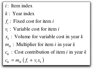
The model used for the cost contribution of item i in
year k is shown below. The cost/time table describes
the multipliers. The fixed cost is in column L and the variable
cost is column O. The result of the computation is not shown
directly on the worksheet but is used to find the cash flow
for each year and the NPW for each item.
Although we see mostly 1's in this matrix, the
coefficients can be altered to represent changes with time.
For instance, if the costs are increasing with inflation, the
numbers in the columns will grow as the year index increases.
A column is included for time 0. This is the
start of the life cycle and any initial investments can be
placed in this column. For the example we see a lone 1 for
item 16, representing the capital cost of the line. Although
the capital cost is spread over several months as illustrated
on the capital budgeting page, for this larger time horizon
we usually place the capital cost at time 0. If, in fact, the
capital cost spreads over several years, the contribution in
each year is indicated by the multipliers.
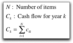
The other columns are for the 6 years of the
product's life. At the top of each year we see the production
volume for that year. The data indicates that this quantity
varies with time. The cash flow at the bottom of each column
is found by summing the item contributions for the year.
The table below summarizes production
amounts and cash flows for the example. We see that except
for time 0, there is a profit for each year in the life. This
cash flow is typical for a profitable investment. The total
cash flow indicates that this system does yield a profit over
its life.
Year |
Prod. |
Cash Flow |
0 |
0 |
$308,000 |
1 |
5,000 |
61,539 |
2 |
8,000 |
98,463 |
3 |
12,000 |
147,695 |
4 |
7,000 |
86,155 |
5 |
4,000 |
49,232 |
6 |
1,000 |
12,308 |
| Total |
37,000 |
147,392 |
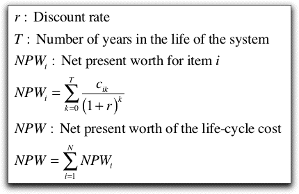
The NPW column computes the present worth for
each item. The present worth computation combines the individual
cash flows into a single equivalent value at time 0. It depends
on the discount rate that must be given. When the discount
rate is 0, the NPW is simply the sum of the cash flows for
an item. The formulas computing the quantities in NPW column
are below.
The NPW worth is used to evaluate the profitability
of an investment. When the NPW is greater than 0, the rate
of return for the investment is greater than the discount rate.
When the NPW is less than 0, the rate of
return for the investment is less than the discount rate. |
Summarize |
| |
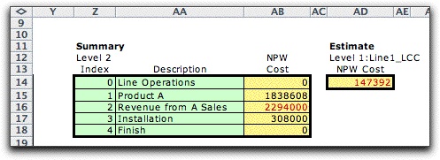
Two
buttons are placed on the life-cycle cost worksheet. One allows
the number of items to changed. The second creates a summary
form that computes the NPW for each set of items having the
same level 2 designation. For the example, the summary shows
the breakdown between operating cost, revenue and installation
cost. Again since we are using zero for the discount rate,
the NPW values are the sums of the costs. The total cost estimate
is shown at the right. Because the value is colored red, it
is negative. This means that the assembly line yields a profit
over its life.
|
The Three Product Example |
| |
The example has three
products: A, B and C. The CBS for this case lists the costs and
revenues for all three products. Click on the icon to see the
CBS in a separate window. Note that we show the product mix in
the N2 column. An item in this case is one unit of product. |
|
| |
The figure below adds
time to the analysis. |
|
| |
The cash flow values are taken from the bottom
of the chart.
Year |
Prod. |
Cash Flow |
0 |
0 |
$308,000 |
1 |
5,000 |
67,042 |
2 |
8,000 |
107,267 |
3 |
12,000 |
160,900 |
4 |
7,000 |
93,858 |
5 |
4,000 |
53,633 |
6 |
1,000 |
13,408 |
| Total |
37,000 |
188,109 |
The summary for this system is below. With three
products the total profit is greater than with only one.

|
| |
The
flexible data structure the Estimate add-in
can be used to estimate the life-cycle cost for a variety of
situations. |
| |
|
|
