 |
There are many risks associated with the estimates regarding
a project, but the add-in only considers the risks associated
with the costs of the work packages. We model the risk by providing
the probability distribution for each work package. Computations
for the distributions are provided by the Random
Variables add-in. This add-in must
be installed for the risk feature to work. As we will see,
the add-in allows computations of probabilities associated
with the project cost. We can compute these using probability
analysis or Monte Carlo simulation.
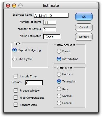
To create a model with risk, fill in the dialog as below.
To keep the illustration simple we use only the first level
of detail for the project, but the analysis can be done for
any level of detail. We have also chosen to not include time,
but that option is available. We have chosen Distribution for
the items amount option. Several distributions are
available, and we have chosen to use the triangular distribution.
In fact, using the General option allows any parametric
distribution allowed by the Random Variables add-in.
The list of the distributions is found on the distributions page
of the add-in. |
| |

|
| |
The work breakdown
structure is constructed as before, but now rather than a single
value for the costs, the name of the distributions and their
parameters are entered in columns E through H. Only the first
three letters,
Tri, are necessary to describe the distribution. The
triangular distribution has three parameters, minimum,
most likely,
and maximum. Other distributions are entered in the
same way, with perhaps different parameters. If the activities
have different distributions, the separate distributions are
described by name.
We see in cell B8 the method by which the point estimates
of the activity times are to be selected. In the present case
we use the mean value of the distribution. The other
options are shown later on this page. The percentile in
B9 has no bearing on the mean value option. |
| |
|
| |
The figure below shows
the computations for the moments of the activity costs.
Column L shows point estimates of the costs, in this case
the mean values. |
|
| |
We show the contents
of some of the cells in row 15. The functions used
in columns I and J are evaluated by the Random Variables add-in,
so that add-in must be installed. The point estimates in column
L are the same as column I, the mean values. |
Summary |
| |
Clicking the Summarize button at the top of the
page summarizes the statistical parameters of the distributions
of the activities at the first level of detail. The mean and
variance values are sums over the parameters of the work package
means and variances. The sum operation is appropriate when
we assume that the work package costs are independent random
variables. Column S shows point estimates for the activity
costs and cell X14 shows the cost of the entire project. |
| |
|
| |
Unless we assume that
all costs are Normally distributed, the distribution of the sum
of the random values is not known. When there are many activities
that together comprise the project, it is reasonable to
assume that the project estimate is normally distributed. Then
we can use the Normal distribution to compute probabilities
regarding this cost. We also can simulate the project cost
as described below. |
Percentile Option |
| |
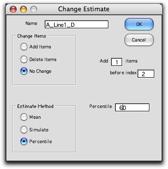
Clicking the Change button
at the top of the page brings the Change Dialog shown
below. The dialog allows the user to add or delete activities,
but in this case we change the estimation method to the percentile method.

|
| |
The data table is the
same except the equation used to select the point estimate in
column L. Now we use the RV_Inverse function. This returns
the value of the activity cost that will exceed the actual
value 60% of the time. It is a conservative estimate since it
is larger than the median value. A percentile of 50% returns
the median, and a percentile less 50% returns a number that is
less than the median. Cell B8 holds the percentile used and can
be changed. B7 holds the word "Percent" indicating that this
is a percentile estimation. |
|
Simulation |
| |
The simulation estimation
method replaces the formulas in column L by the RV_Sim function.
This function simulates a value using the Monte Carlo method
for the distribution defined by its argument. Every time the
worksheet is computed new simulated values are obtained and the
summary ranges that relate to the point estimate also change. |
|
| |
The simulation option
is not of much value by itself, but it allows the user to simulate
the total project cost using the Simulation option
of the Random Variables add-in. The dialog below is called by
choosing the Simulate_RV item from the ORMM menu. The
simulated cell is the X14. This cell holds the total cost of
the project. The statistics to be computed are selected by
checking the boxes on the dialog. We ask for a simulation of
500 observations. |
| |
|
| |
The worksheet is recomputed
500 times and statistics associated the value
in cell X14, the project cost, are accumulated. They are shown
on the worksheet starting in Y14. The simulated mean and variance
are close to the theoretical mean and variance in cells
U14 and V14. |
| |
|
| |
The histogram generated
by the add-in is below. It is similar to a typical
bell-shaped curve (the Normal distribution), but it is skewed
to the right. This is not unexpected since all the triangular
distributions were skewed to the right. |
| |
|
| |
Other measures related
to the project cost can easily be computed using features of
the Random Variables add-in. |
Time |
| |
The time option
is also available for the models with risk. In that case the
summary will describe the statistics for the net present worth
of the project. |
| |
|


