This game involves the stochastic inventory situation illustrated in the figure above. This example uses the (q, r) policy to control the inventory. The inventory level is affected by demands and replenishments, but the demand process is variable. Sometimes the demand is high causing quickly declining inventory levels, while at other times the demand is low with the inventory declining more slowly. For this system, we have some inventory level r at which we place an order for an inventory replenishment. This is called the reorder point. The amount ordered is q, the order quantity. After we place the order, we must wait for some interval, L, the lead time, before the inventory is replenished. Because of the variable demand and the lead time, there is a risk that shortages will occur. In the figure, the shortages are shown as the red areas. If the demand is high during the lead time (greater than r), some customers will not be satisfied. For this game we assume that shortages are backordered. Eventually as supply becomes available the backordered demand is satisfied. We can set the reorder point high to make shortages unlikely, but that will increase the inventory levels, shown as the blue areas. The order quantity affects both shortages and inventories as well as the cost of replenishment. The game player plays the role of the inventory manager. The goal of the game is to minimize the total cost of operating the inventory.

The simulated model used for the game is slightly different than the situation pictured in that the inventory is observed weekly and orders can be placed only at the end of a week. This is called discrete review. The picture shows continuous review where orders can be placed at any time. In our model, at the end of each week the player must decide to order or not. If a nonzero order quantity is chosen, that quantity arrives L weeks later at the beginning of the week. The parameters of the model are shown to the left of the figure. Demand is a random variable governed by a normal distribution with given mean and standard deviation. All these parameters can be changed, but we use the parameters above for the example on this page.

To start playing the game press the Start button on the Start_BO worksheet.

A dialog opens to accept the inventory parameters and stores them on the game worksheet. The parameters become the default values for the next play of the game.

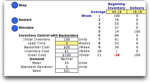
Clicking the OK button on the Initial Conditions dialog opens the Inv_BO worksheet where the game is played. The figure below shows the worksheet as it first appears. In addition to the control buttons, the dialog at the upper left holds the step number, a description of the decision to be made and the order quantity field. Step 1 requests the order quantity decision for at the end of the first week.

The simulation starts at the end of week 1. The data for week 1 is shown in the row labeled 1. The beginning inventory of week 1 is set as an initial condition. The demand for week 1 is randomly generated from a normal distribution with mean 25 and standard deviation 5 (rounded to an integer and truncated to a non-negative number). The first week's simulated demand is 24. There are no deliveries in the first week. The ending inventory is the beginning inventory plus the deliveries minus the demand. Shortages are backordered and a shortage condition is indicated by a negative value for the ending inventory. The yellow line just above the row for week 1 holds the averages or mean values of the columns.

Only the order quantity field is controlled by the user. In the example, we choose to order 100 units at the end of period 1. The order will be delivered at the beginning of week 5 since the lead time is 3 weeks. Three full weeks pass before the delivery, weeks 2, 3 and 4.

The Next button leads to the next week. The Quit button temporary suspends time.

We continue the example for 11 weeks and the add-in constructs the table showing the order quantity decisions and the corresponding results. Summary results are shown to the right. The Quit button on the game dialog leaves the worksheet in this intermediate state allowing the game player time for analysis and planning. Note that the game encounters are backorder situation at the end of week 10. The delivery in week 11 accommodates the backorder and satisfies the demand of 32, leaving 40 units in inventory.

The game buttons at the top left of the worksheet control the simulation. Clicking the Step button resumes the simulation at week 11. The Restart button returns the game to first week. The parameters remain the same. The Simulate button replaces the random number seed with one created with the Excel random number generator. The effect is to obtain a different sequence of random demands. The Simulate button is particular useful for evaluating policies with different demand patterns.

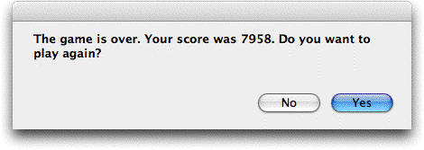
We continue the example until 52 weeks pass. The game ends with the message below.

The display shows the 52 weeks of the game along with the summary results as shown below.

The complete history of the 52 week game is shown below. For illustration we used a variety of order quantities. Over 12.5% if the demand requests were backordered. With practice, you can do much better.

Once the game is complete, clicking the simulation button changes the sequence of random demands. The figures below show the results of four simulations using the policy derived for the example. Generally, a solution derived for a specific sequence of demands does not work very well for others. For our case the first two demand patterns worked better for the solution, while the last two did worse. This probably reflects on the poor quality of the solution provided for this example.