|
|
 |
Inventory Game |
 |
-
Lost Sales |
|
|

This model is similar to the Backorder case except
whenever the inventory is exhausted, sales of subsequent demand
is lost until the next delivery arrives. There is a specified
cost for each lost sale. The goal is to place replenishment
orders to minimize the total cost of orders, inventory and
lost sales. Since revenues from sales and costs of purchasing
the item is not included, the lost sales cost must reflect
the lost profit plus any penalties for losing the customer.
The simulated
model used for the game is slightly different than the situation
pictured in that the inventory is observed weekly and orders
can be placed only at the end of a week. This is called discrete
review. The picture shows continuous review where orders can
be placed at any time. In our model, at the end of each week
the player must decide to order or not. If a nonzero order
quantity is chosen, that quantity arrives L weeks
later at
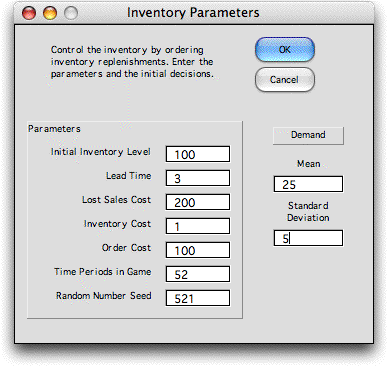
the beginning of the week. The parameters of the model are
shown to the left of the figure. Demand is a random variable
governed by a normal distribution with given mean and standard
deviation. All these parameters can be changed, but we use
the parameters above for the example on this page. |
| Start |
| |
To start playing the game press the Start button
on the Start_LS worksheet.

A dialog opens to accept the inventory parameters
and stores them on the game worksheet. The parameters become
the default values for the next play of the game.

|
| Play |
| |
Clicking the OK button
on the Initial Conditions dialog opens the Inv_LS worksheet
where the game is played. The figure below shows the worksheet
as it first appears. In addition to the control buttons, the
dialog at the upper left holds the step number, a description
of the decision to be made and the order quantity field. Step
1 requests the order quantity decision for at the end of the
first week.
The display is similar to the backorder display
with the exception of a new column for Lost Sales.
Because shortages are not backordered, the ending inventory
never goes below zero. The new column is used to record and
evaluate the cost of lost sales.
The Next button leads to the next week.
The Quit button temporary suspends time. |
|
| |
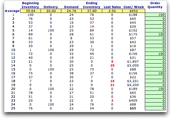
We figure below shows the results
of 25 weeks of play. The first instance of lost sales occurs
at week 13. The initial inventory is 21, there are no deliveries,
and the demand is 30. The resulting final inventory is 0 and
9 sales are lost. The cost for the week is $1807. This includes
$1800 for the lost sales ($200 each) and $7 for the average
inventory during the week. |

|
| |
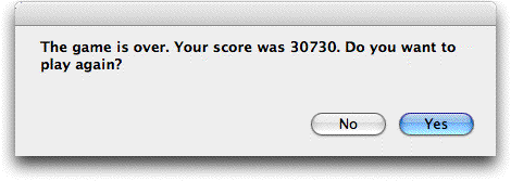
We continue the example until 52 weeks pass. The game ends
with the message below.

An answer of No to retains the results.
An answer of Yes resets the results to week 1. The
summary below shows that the solution provided by the author
lost over 10% of the demand due to shortages.

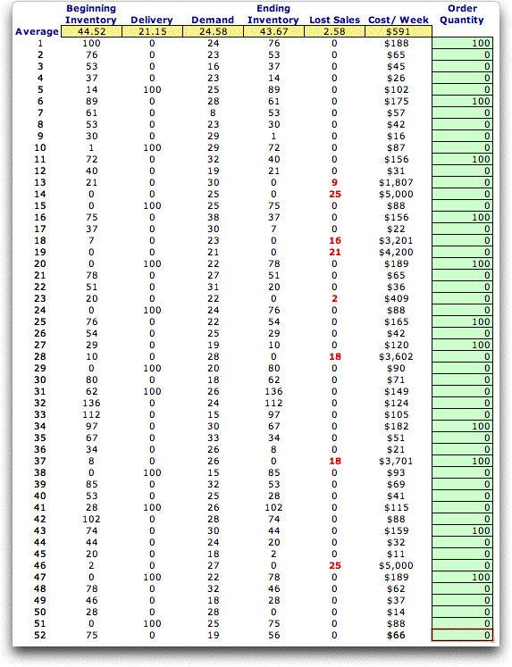
The complete history of the 52 week game is
shown below. With practice, you can do much better. One interesting
difference from the backorder case is the difference between
the average delivery and the average demand. Since part of
the demand is lost the total deliveries will usually be less
than the total demand. For a finite game the initial and final
inventories also affect this relationship. |

|
| Simulate |
| |
Since this game is very similar
to the Backorder game, we will not repeat the sections
on simulation. The Simulation button, changes the
seed for the random demand so that a specified policy can be
evaluated for different demand streams.
|
|
| |
|
|


