The moving average forecast is based on the assumption of a constant model.

We estimate the single parameter of the model at time T as average of the last m observations, where m is the moving average interval.

Since the model assumes a constant underlying mean, the forecast for any number of periods in the future is the same as the estimate of the parameter:

In practice the moving average will provide a good estimate of the mean of the time series if the mean is constant or slowly changing. In the case of a constant mean, the largest value of m will give the best estimates of the underlying mean. A longer observation period will average out the effects of variability.

The purpose of providing a smaller m is to allow the forecast to respond to a change in the underlying process. To illustrate, we propose a data set that incorporates changes in the underlying mean of the time series. The figure shows the time series used for illustration together with the mean demand from which the series was generated. The mean begins as a constant at 10. Starting at time 21, it increases by one unit in each period until it reaches the value of 20 at time 30. Then it becomes constant again. The data is simulated by adding to the mean, a random noise from a Normal distribution with zero mean and standard deviation 3. The results of the simulation are rounded to the nearest integer.

The table shows the simulated observations used for the example. When we use the table, we must remember that at any given time, only the past data are known.

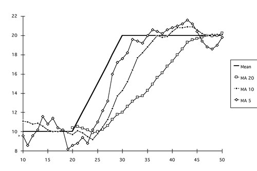
The estimates of the model parameter, , for three different values of m are shown together with the mean of the time series in the figure below. The figure shows the moving average estimate of the mean at each time and not the forecast. The forecasts would shift the moving average curves to the right by periods.

One conclusion is immediately apparent from the figure. For all three estimates the moving average lags behind the linear trend, with the lag increasing with m. The lag is the distance between the model and the estimate in the time dimension. Because of the lag, the moving average underestimates the observations as the mean is increasing. The bias of the estimator is the difference at a specific time in the mean value of the model and the mean value predicted by the moving average. The bias when the mean is increasing is negative. For a decreasing mean, the bias is positive. The lag in time and the bias introduced in the estimate are functions of m. The larger the value of m, the larger the magnitude of lag and bias.

For a continuously increasing series with trend a, the values of lag and bias of the estimator of the mean is given in the equations below.

The example curves do not match these equations because the example model is not continuously increasing, rather it starts as a constant, changes to a trend and then becomes constant again. Also the example curves are affected by the noise.

The moving average forecast of periods into the future is represented by shifting the curves to the right. The lag and bias increase proportionally. The equations below indicate the lag and bias of a forecast periods into the future when compared to the model parameters. Again, these formulas are for a time series with a constant linear trend.

We should not be surprised at this result. The moving average estimator is based on the assumption of a constant mean, and the example has a linear trend in the mean during a portion of the study period. Since real time series will rarely exactly obey the assumptions of any model, we should be prepared for such results.

We can also conclude from the figure that the variability of the noise has the largest effect for smaller m. The estimate is much more volatile for the moving average of 5 than the moving average of 20. We have the conflicting desires to increase m to reduce the effect of variability due to the noise, and to decrease m to make the forecast more responsive to changes in mean.

The error is the difference between the actual data and the forecasted value. If the time series is truly a constant value the expected value of the error is zero and the variance of the error is comprised of a term that is a function of and a second term that is the variance of the noise, .

The first term is the variance of the mean estimated with a sample of m observations, assuming the data comes from a population with a constant mean. This term is minimized by making m as large as possible. A large m makes the forecast unresponsive to a change in the underlying time series. To make the forecast responsive to changes, we want m as small as possible (1), but this increases the error variance. Practical forecasting requires an intermediate value.

Forecasting with Excel

The Forecasting add-in implements the moving average formulas. The example below shows the analysis provided by the add-in for the sample data in column B. The first 10 observations are indexed -9 through 0. Compared to the table above, the period indices are shifted by -10.

The first ten observations provide the startup values for the estimate and are used to compute the moving average for period 0. The MA(10) column (C) shows the computed moving averages. The moving average parameter m is in cell C3. The Fore(1) column (D) shows a forecast for one period into the future. The forecast interval is in cell D3. When the forecast interval is changed to a larger number the numbers in the Fore column are shifted down.

The Err(1) column (E) shows the difference between the observation and the forecast. For example, the observation at time 1 is 6. The forecasted value made from the moving average at time 0 is 11.1. The error then is -5.1. The standard deviation and Mean Average Deviation (MAD) are computed in cells E6 and E7 respectively.