|
|
 |
Functions |
 |
-
Integrate |
|
To integrate a function, choose Integrate from
the menu. Three numerical methods are provided: Simpson's Rule,
the Monte Carlo method and the Quasi Monte Carlo method. Simpson's
Rule is available when the number of integration variables
is four or less. The Monte Carlo method can be used with any
number of integration variables. The Quasi-Monte Carlo method
is available with twenty or fewer integration variables. For
a given number of function evaluations, the accuracy of all
the methods is seriously degraded as the number of integration
variables increases. To obtain more accuracy with multiple
dimensions requires a great many observations. Since the two
Monte Carlo methods involve random selection of the points
to be evaluated, these methods provide statistical measures
of the accuracy of the estimated integral value.
Most of the results of this page come from Methods of
Numerical Integration, (Davis, P. J. and Rabinowitz,
P., 2nd ed. New York: Academic Press, 1984), or from personal
communications with David Morton from the University of Texas
who inspired this part of the add-in. |
| |
|
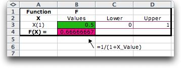
For the first example, we use a simple function with
a single decision variable, the same one considered on
the summary page.
The form describing the function is shown
in the picture.
|
|
| |
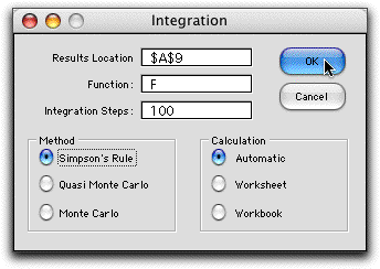
The Integration dialog
selects the function to be integrated, the location of the
integration results, the number of steps in the integration,
the integration method, and the strategy for performing calculations.
The first page of this section
describes the Calculation options. For small dimensionality
problems with simple functions, the Automatic option
is probably the best. When using this add-in it is important
to set the Excel Calculation option, set in the Preference dialog,
to Automatic. |
Simpson's Rule |
| |
For the example,
the integral can be computed exactly as:
Simpson's Rule evaluates the function in the range
[a,b] with points at a and b
with the remaining points equally spaced in the interval. There
are 2n intervals and 2n + 1 the evaluation
points.
The results of Simpson's Rule with 100 observations for the
example are shown below. The program does not count the observation
at the lower bound, so there are actually 101 observations.

The numerically obtained results are quite close
to the correct value with 100 observations. Simpson's Rule is
generally satisfactory for functions of a single variable when
the function has continuous derivatives. With a single-dimensional
quadratic function, 3 observations (n = 1 in the expression
above) yields an accurate solution since Simpson's rule is based
on a piece-wise quadratic approximation. |
Monte Carlo Method |
| |
An alternative way to estimate
the integral is through simulation. The procedure is called
the Monte Carlo method. To estimate an integral we draw a number
of random observations of the function with the range of the
integration variables and use the average of the observations
as an estimate of the integral. With a single variable of integration,
an observation of the function is determined using a randomly
selected value within the range of the variable.
For the moment assume that the range of integration
is from 0 to 1. To estimate the integral and at the same time
find the variance of the estimate, we divide the total number
of observations into samples of 30. The mean of the observations
is computed for each sample. The grand mean of the 30 sample
means is the estimate of the integral. An estimate of the variance
of integral is obtained from the variance of the sample means.
When the range of integration is not [0,1], the estimate of
the integral and its variance must be adjusted for the range.
Because we have used 30 samples, we can use the consequences
of the Central Limit Theorem to create a confidence
limit.
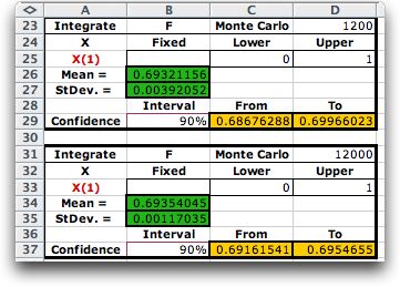
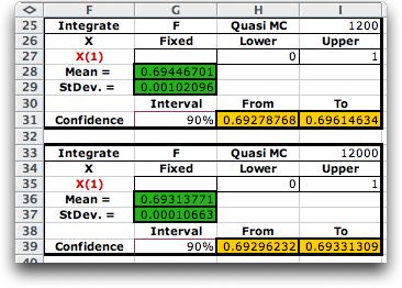
The results for the example are shown for three
different numbers of observations.
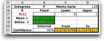
For the Monte-Carlo integration method, observations
of the independent variables are randomly selected, 120 in this
case. The average function value of the observations multiplied
by the range provides an estimate of the integral, presented
shown in cell B18. Since the result is a random variable, we
estimate the standard deviation of the integral estimate, presented
in cell B19. Because of the Central Limit Theorem the
mean of the sample means is approximately Normally distributed,
so we use the Normal distribution to provide a confidence limit
for the integral. The confidence level in B21 can be changed
by the user. Formulas in cells C21 and D21 show the range of
the confidence limit. With a larger number of observations,
the standard deviation of the estimate and the width of the
confidence interval is decreased. To decrease the standard deviation
of the estimate by a factor of 10, the number of observations
must be increased by a factor of 100. This is illustrated by
comparing the standard deviation with 120 observations (0.01156)
with the standard deviation for 12000 observations (0.00117).
|
Quasi-Monte Carlo Method |
| |
The Quasi-Monte Carlo
method generates the values for observations that more equally
distribute the observations in the range of the integration
variables. For a single dimension the formula for the observation
k is:
Quasi-Monte Carlo provides more accurate results
for the same number of observations than the Monte Carlo when
the number of variables is moderate. The add-in limits the number
of integration variables to 20 for the Quasi-Monte Carlo method.
This is a limitation of the program, not the method. The random
number  depends
on the sample number n. It is added to introduce randomness
between samples to allow the computation of the standard deviation.
When modified in this way the method is called Randomized
Quasi-Monte Carlo. depends
on the sample number n. It is added to introduce randomness
between samples to allow the computation of the standard deviation.
When modified in this way the method is called Randomized
Quasi-Monte Carlo.
|
More than One Integration Variable |
| |
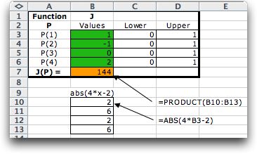
To illustrate integration
over more than one integration variable we use the four dimensional
example below.
The absolute values used in the function make
the first derivatives of the function discontinuous whenever
a variable has the value 0.5. The integral of this function
of the ranges of the four decision variables is:
The add-in integrates over the ranges prescribed
by the lower and upper bounds given on the function form. The
function's representation on the worksheet refers to the calculations
just below the function form.
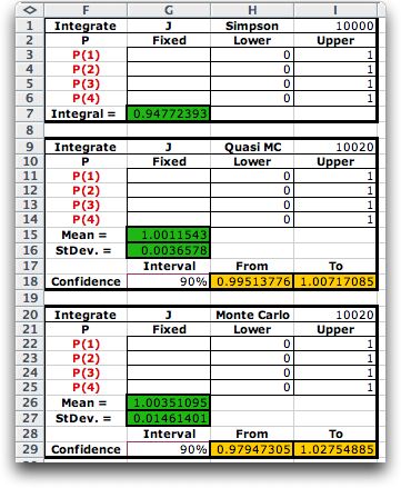
We apply the three integration methods below.
Simpson's Rule is applied recursively to the four variables
of integration. The number of points investigated for each dimension
is the 4th root of 10000 or 10. If the 4th root of the number
of observations is not an integer, the number of observations
is adjusted to obtain an integer value. For this case one would
not expect the Simpson's Rule to give a very accurate answer,
and it does not.
In the case of the Monte Carlo and Quasi Monte
Carlo methods, the number of observation must be a multiple
of 30. When 10000 observations are requested, the program increases
this number to the next higher multiple of 30, 10020. With this
number the methods run 30 samples of 304 observations each (30*304
= 10020).
This function has a complicated shape with discontinuous
first derivatives. We see that Simpson's Rule with 10 observations
per dimension is not accurate. The two Monte Carlo methods provide
90% confidence intervals that contain the true value.
Simpson's Rule is perfectly accurate for quadratic
functions. With a four dimensional quadratic function, the
Rule returns an accurate solution with only 81 observations
(3 per dimension).
 |
Integration over a Subset of Variables |
| |
With multiple variables, it is
possible to integrate over a subset of the variables with the
remainder of the variables fixed at specified values. To fix
a variable give equal lower and upper bounds to the variable
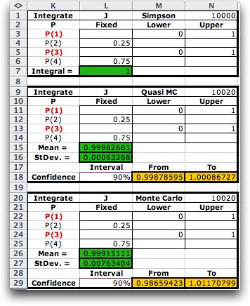
in the function form. The example shows P(2) fixed at 0.25 and
P(4) fixed at 0.75. These values make the factor for each of
these terms equal to 1 in the function.

Integration is over the remaining variables. In
the results shown below, Simpson's Rule provides the exact result
(the exact integral has the value 1). With only two remaining
integration variables, Simpson's Rule has 100 observations for
each dimension. The Monte Carlo results are also more accurate
because of the reduced dimensionality of the integral. In the
result below, the names of the integration variables are colored
red and the fixed values are shown in column L.
|
Application |
| |
One important application of integration
is computing the expected value of some measure that depends
on random variables.
Here the integrations are performed over the ranges
of the random variables.
For simulation studies, some measure of effectiveness
is defined for the simulated system and a model is constructed
that relates the measure to parameters of the system. When some
parameters are random variables, the model uses random number
seeds for each random variable. A simulation run with a specified
set of seeds, one for each random variable, gives a single observation
of the measure. The goal of the simulation study is to determine
the expected value of the effectiveness measure. To do this
requires an integration as described on this page. The seeds
are chosen from uniform distributions that range from 0 to 1.
As illustrated by some of the examples, integration
in multiple dimensions is not always easy. Since the functions
computed by simulation are often very complex, many observations
may be required to obtain accurate results. |
| |
|
|


