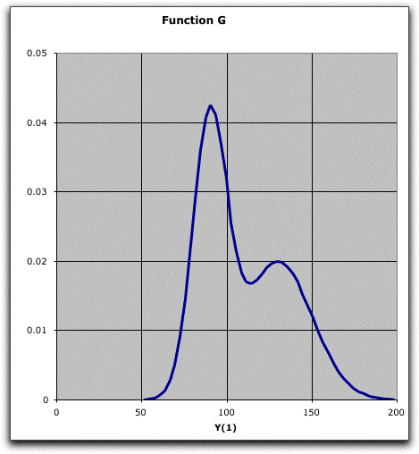
A graph of the function shows two peaks. This might describe a mixture of two separate populations. The graph was created by the add-in.

This is not a true probability distribution because the area under the function is not 1, but rather approximately 2. We have truncated the distribution so that the entire mass lies between 50 and 200.

Although it may be possible to analytically determine the moments of this distribution, the add-in uses numerical integration to compute them. A dialog presented by the Moments command accepts data for the results location for the display, the name of the function, the variable index (important when there is more than one variable), the integration method, and the calculation option. The integration steps is the number of observations for the numerical integration. The plotting steps is the number of points that will be included in the plot of the function. The number of moments determines how many will be computed or displayed. The number must be between 1 and 4. Checkboxes determine whether moments and/or plot are displayed.

Moments computed with Simpson's Rule from 50 observations are placed on the worksheet.

The exact moments have the following definitions. We use f for the general function and x for the general variable. The variable is bounded by a and b.

If the function is a probability distribution, the constant term is 1. Otherwise the constant term adjusts the distribution for the calculation of the moments. The mean, variance and standard deviation are well known characteristics of distribution functions. The skewness, as indicated by Beta(1), measures the symmetry of a distribution. Symmetric distributions have a skewness of 0. If the mass of the function is concentrated to the left of the mean and the distribution has a tail that decreases to the right, the skewness is positive, as for the example. Negative skewness indicates that the greater mass is to the right and the tail is to the left. The kurtosis measures the relative thickness of the tails of the distribution. The value of Beta(2) is 3 for a Normal distribution.

The add-in approximates the integrals associated with the moments using one of the numerical integration methods. When one of the Monte Carlo methods is used, estimates of the error variance are obtained and used to construct confidence intervals for the moments. The confidence intervals for measures computed by combining moments are difficult to calculate and are not presented. The intervals change with the Confidence value in cell B24. Since all the integrals use the same observations, estimates of the different moments are not independent.

The Moments dialog provides an opportunity to plot the function. The plotting program collects the functional values used to compute the moments. The range is divided into a number of intervals and the average function value within each interval is computed. Points are plotted at the mid-points of the intervals. The graph below is constructed for the example using Monte Carlo sampling with 1020 observations divided into 50 intervals. For the Monte Carlo methods, there must be many more observations than intervals for a smooth graph. When using Simpson's Rule with one dimension, the number of observations must be no less than the number of intervals for the graph.

More than One Dimension

To illustrate moments for functions with more than one dimension, consider a bivariant Normal distribution.

This equation does not include the constant term. The add-in computes the constant and uses it to adjust the results. The formula for the function is in cell B5 of the function form. Although the range of the bivariant Normal distribution is unbounded, we set lower and upper bounds that are three standard deviations from the mean. The add-in requires bounded variables.

In the Moments dialog, we specify the variable index as 2. Moments will be calculated for the second variable (y). When computing moments, any one of the variable indices may be chosen.

The equation for the constant and mean of y are double integrals. The other moments are similar. The moments are for the marginal distribution of y.

The add-in approximates the moments for y by estimating these integrals and presents the results on the worksheet. It happens that the marginal distribution for y is also a Normal distribution. The Normal distribution has Beta(1) = 0, indicating that the distribution is symmetrical. The estimated value of Beta(1) is small. All Normal distributions have Beta(2) = 3. The sampled data has Beta(2) = 2.83. The difference from 3 is partly due to the truncation of the Normal distribution with finite bounds.

The plot of the function is shown below together with part of the table from which the plot is derived. Although the exact distribution is a Normal distribution, the plot is determined from the 10020 observations used to compute the mean. The Quasi Monte Carlo method puts approximately the same number of observations in each plot interval. The chart is bumpy because of the statistical nature of the data.

Moments for the Conditional Distribution

With multiple variables, it is possible to fix some of the variables and find the moments for the conditional distribution of the remaining variables. For the example, we fix the value of x to 0 by setting both the lower and upper bounds to 0.

On the worksheet range showing the moment results, the fixed variable is shown in black and the integration variable is shown in red. The moments are computed for the conditional distribution of y|x = 0.

The results for the conditional distribution are more accurate and the graph is smoother than for the marginal distribution, because with x fixed there is only one variable of integration, and over 10000 observations are used to calculate the moments and construct the graph.

Moments can be calculated for any non-negative function. Functions with negative values do not represent probability distributions and moments will not be computed. The plotting option works for all functions with bounded value.

Application

The moments of a variety of named probability distributions are well known and are easily calculated. Use the Random Variables add-in for finding the moments of the sixteen different named continuous and discrete distributions described there. The moments for more general distributions are difficult to obtain. When closed form equations define a distribution, it may be possible to analytically derive expressions that calculate moments for general parameters, but in many cases, especially those that involve more than one variable, general expressions are difficult if not impossible to find. Otherwise, it is necessary to use numerical integration as provided by this add-in. This is certainly necessary if the distribution is not a closed form expression, but is provided by complex computations in an Excel workbook.

When a function is not a probability distribution function or does not have a closed form, it might also be interesting to compute moments. For example, a function may describe some measure for a system that depends on several control parameters. We might be interested on how one parameter affects the measure when one integrates over all the rest. Estimation of the moments for the one parameter will suggest the best value of the parameter or the variability of the response to that parameter.