With the no recourse situation, we must fix the decision variables before the random variables are realized. On this page we investigate some simple strategies for finding solutions. We will finally conclude that these strategies are not very satisfactory. The following pages suggest better, but more difficult, solution methods.

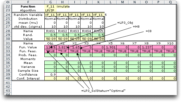
One strategy is to replace the random variables by their expected values and solve the resultant deterministic model. We might ask how well this expected value solution serves as the solution to the stochastic problem. The expected value solution to our example problem is shown below. Since the expected values of the random variables are 0, the RHS values are just the constants originally proposed.

To evaluate this solution in a stochastic setting, we create a different model below. The LP model is the same as before, but now we allow the RHS values to vary randomly but do not solve the LP for each sample. For each sample, the solution is fixed at the deterministic solution obtained with the expected RHS. The objective value does not change because the decision vector is fixed. The only question is what is the probability that this solution will be feasible?

We have placed logical expressions in G15:G19 to indicate when the constraints are feasible. In the function form below, cell G33 contains a logical expression that is TRUE only when all constraints are all satisfied. The LP solution on the worksheet is optimal when the RHS takes the expected value, so this solution is feasible.

These results should not be surprising. With the expected RHS values, four of the five constraints are tight in the deterministic optimal solution. Since the RHS values are Normally distributed, there is a 50% that a tight constraint will be violated when the random RHS is realized. Even if the single loose constraint is never violated, the probability that all the tight constraints are satisfied is 0.5 raised to the fourth power or 0.0625. The simulated result is quite close to this value.

One might ask, how should the problem with no recourse be solved? The answer to this question is the provence of stochastic programming.

Combining Wait and See Solutions

One suggestion often made for this kind of problem is to solve the problem as if we could wait and see the random realizations and then combine the wait-and-see decisions in some way. We do this for the example by creating a new math programming model identical to the wait and see model considered earlier, but create a simulation form that records the values of the decision variables as well as the objective. The form is below. We now have 11 functions defined. The first is the objective function and the remaining ten are the values of the decision variables. All eleven functions have the same feasibility equation. A solution is recorded only when the LP has a feasible solution.

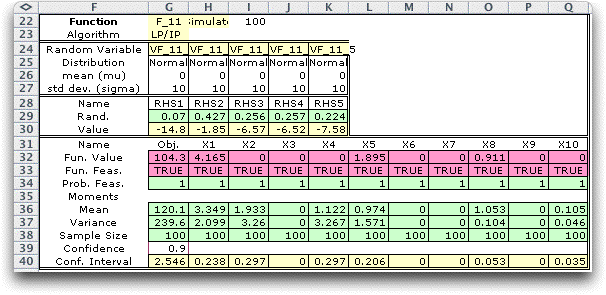
We simulate the random variables, solve the LP for each sample point and record the observed function values. The results from 100 observations is below. Row 36 shows that six of the decision variables have non-zero values in some of the observations.

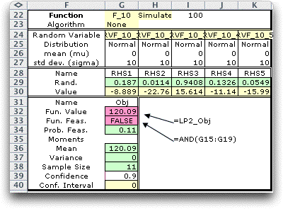
To continue, we impose the average-decision-value solution shown in row 36 on the LP model.

To evaluate this solution, we simulate this model with the solution fixed as above. Of course, since the solution is fixed there is no variability in the objective function. The results indicate that the solution is feasible for 11% of the simulated RHS vectors.

We have investigated two solutions to the no-recourse problem, the expected value solution and the mean wait-and-see solution. The two solutions are shown in the table. When uncertainty affects the RHS values of the constraint coefficients, there is always a chance that some constraints will be violated by a fixed solution. Choosing a solution involves a tradeoff between the risk of infeasibility and the expected value of the objective function. Chance Constraints, described on the next page, gain some control of the feasibility probability, but again we will be left with a variety of solutions to choose between.