When it is necessary
to make decisions in a situation that involves uncertainty,
it is always good to have recourse. In the recourse situation
some of the decisions must be made before the uncertainty
is
realized and then other decisions, the recourse decisions,
can be made after the values of the random variables are known.
The model has two stages as described below. We use notation
that is compatible with the side-model notation introduced
earlier. For this discussion we restrict attention to the linear
case. The first-stage decisions are the vectors x and z.
The decisions x appear only in the first-stage
model, while z links the first and second
stage. These
decisions are constrained by linear constraints and simple
upper bounds.
The first-stage decisions contribute directly to the objective
value
through
the first-stage costs.
The random variables affecting the second
stage are described
by the vector  .
In the most general case the vector may affect all aspects
of the second-stage problem as indicated by the
tildes over the parameters of the second stage. The cost of
the second stage, .
In the most general case the vector may affect all aspects
of the second-stage problem as indicated by the
tildes over the parameters of the second stage. The cost of
the second stage,  ,
depends on z and on the realization of ,
depends on z and on the realization of  .
This cost is a random variable. The problem for the decision
maker is that x and z must
be set before the realization, so the most reasonable first-stage
decision should minimize the first-stage cost plus the
expected value of the second-stage cost. .
This cost is a random variable. The problem for the decision
maker is that x and z must
be set before the realization, so the most reasonable first-stage
decision should minimize the first-stage cost plus the
expected value of the second-stage cost.
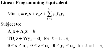
It has been shown that there is a linear programming
equivalent to the two-stage model when there is a finite
number of possible realizations of the random features
of the second stage. We call a particular realization
a scenario and index the second-stage components to identify
the scenarios. Each scenario has a specified probability.
The solution of the linear programming model simultaneously
determines the first-stage decisions and the second-stage
decisions for
all scenarios. The last term in the objective function computes
the expected recourse cost.
The fact that we can solve the stochastic programming problem
with recourse is good news, since packages are available to
solve large models efficiently. The difficulty is that for
even small stochastic problems, the models become very large.
The free Solver that comes with Excel can handle no more
than 200 variables. Only very trivial problems
are this small. We illustrate the method with a very small
problem below and for a larger problem on the next page.
In the remainder of this section we consider only problems
that can be modeled with the side model feature of
the Math Programming add-in. We can build much larger models
than can be solved with the free Solver. Solver versions with
much larger capacities can be purchased from Front-Line Systems.
With the side model, the matrix W must be
the same for all realizations.
Although the general model includes a matrix Tk that
depends on the scenario index k, we restrict
attention to those allowed by the side model
feature. Here a square diagonal matrix Dk is
defined for each scenario. In the constraint set the diagonal
matrix post multiplies a constant matrix T. Since
only the diagonal elements are relevant they are stored on
our side-model form in a single row for each scenario.
Although not every situation can be handled using these matrices,
we will
find
that they
are very useful for some applications. For applications where Tk does
not vary by scenario, Dk is
an identity matrix for all k. The feature is illustrated
for a two variable example below.
With these limitations, the problems to be considered
are below.

More general models are easily constructed
with the Math Programming add-in that allows inequality constraints,
simple lower bounds, integer variables and various kinds of
nonlinearities. |


