| |
 |
To illustrate a recourse problem, we consider a capacity expansion
problem that has the form of a transportation problem. This example
was contributed by David Morton at the University of Texas.
A company will supply electricity to three demanders from
two electric generators. The unit cost of supplying each customer
from each generator site is given below.
Transport Cost
|
Dem. 1
|
Dem. 2
|
Dem. 3
|
Gen. 1
|
4.3
|
2
|
0.5
|
Gen. 2
|
7.7
|
3
|
1
|
The amounts required by the three demanders is uncertain.
Each demand has three levels with amounts and probabilities
given below. The probability distributions are independent.
Demand/ Probability
|
Dem. 1
|
Dem. 2
|
Dem. 3
|
Level
|
|
|
P(  )
|
|
|
|
P(  )
|
|
|
|
P(  )
|
|
|
|
|
|
|
|
2
|
|
|
|
|
3
|
|
|
|
To supply the electricity, the company will install capacity
at the two generators. The first-stage decisions are and and  ,
the installed capacity at the two generators. The unit costs
of installed capacity are $400 and $350 at generator 1 and
2 respectively. The total capacity cannot exceed 10,000. ,
the installed capacity at the two generators. The unit costs
of installed capacity are $400 and $350 at generator 1 and
2 respectively. The total capacity cannot exceed 10,000.
The reliability of the installed capacity is uncertain. The
fractions  and and  are
the proportions of the installed capacity that will actually
be available for satisfying demand. There are three levels
of reliability as given in the table. These probability distributions
are independent. They are also independent of the demand random
variables. are
the proportions of the installed capacity that will actually
be available for satisfying demand. There are three levels
of reliability as given in the table. These probability distributions
are independent. They are also independent of the demand random
variables.
Reliability/ Probability
|
Reliability 1
|
Reliability 2
|
Level
|
|
|
P(  )
|
|
|
|
P(  )
|
|
|
|
|
|
|
2
|
|
|
|
3
|
|
|
The decision maker must select the generator capacity to install
before knowing the demand or reliability. The second-stage
decisions are the decisions about which demands to service
from the generators. In the following  is
the demand satisfied at customer j from generator i.
We add a third supplier, Subcontract, to represent
demand not met from the generators. The cost can be viewed
as a penalty cost or as the cost of satisfying the demand through
a subcontractor. is
the demand satisfied at customer j from generator i.
We add a third supplier, Subcontract, to represent
demand not met from the generators. The cost can be viewed
as a penalty cost or as the cost of satisfying the demand through
a subcontractor.
The problem has the form of a transportation model as shown
below with random variables and decisions affecting the supplies
and demands.
Transport Cost
|
Dem. 1
|
Dem. 2
|
Dem. 3
|
Supply
|
Gen. 1
|
4.3
|
2
|
0.5
|
|
Gen. 2
|
7.7
|
3
|
1
|
|
Subcontract
|
6000
|
6000
|
6000
|
no limit
|
Demand
|
|
|
|
|
The transportation model cannot be immediately solved because
its parameters depend on five random variables and two decisions
determined elsewhere. |
The Recourse Model |
| |
To find the optimum
values of the generator capacities, we setup a recourse model. The
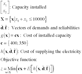
first-stage problem is to select capacities for the generators.
First-Stage Model
|
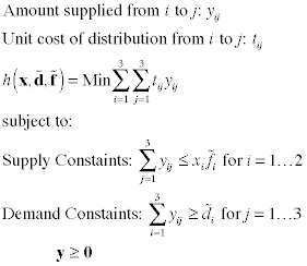
The second-stage problem is to distribute the electricity.
Second-Stage Model
|
The two models can be combined to form a deterministic linear
programming model that represents all 243 combinations of
the
random variables explicitly. This model has 2,189 decision
variables and 1,216 structural constraints. The free Solver
that comes
with Excel is not able to solve a problem of this size, but
it is possible to set the problem up using the Math
Programming
add-in.
The problem may be solved with the L-shaped method available
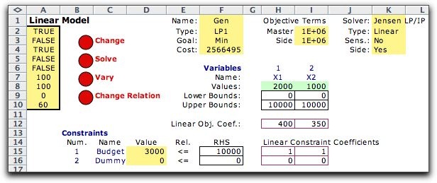
through the Jensen LP/IP add-in. The master problem describes
the variables for the generator capacity
and the
limit on the
maximum
capacity.
The
second
constraint shown is irrelevant. The arbitrary solution (2000,1000)
is shown for illustration.
The side model has a row for each scenario. To
reduce the width of this page we show the model in two parts.
Only 20 submodels are shown, but there are 243 in total. The
part of the model representing the transfer variables (generator
capacities)
and subproblem
variables
(distribution
decisions) is shown below. By clicking the Solve button
on the side model form, the submodels are optimized and the
optimum solution is shown for the master problem solution (2000,
1000). |
|
| |
The remainder of the form shows the constraints
of the subproblems. The relations are entered in row 32. The
RHS values are different for each scenario and are prescribed
in columns AD through AH. The yellow fields in columns Y through
AC show the value of each constraint for the current solution.
Comparing the constraint values to the RHS values will show that
all subproblem solutions are feasible. |
| |
|
| |
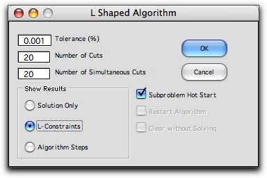
When the Solve button at the right
of the master problem is clicked, the add-in presents the L-shaped
algorithm dialog. We have chosen to see the optimality constraints
with the final solution.
After 13 optimality cuts and 7345 simplex iterations
requiring 17 seconds on the author's computer we obtain the solution
below. This is not the optimum because a gap of 2.66 remains between
the lower and upper bounds. |
|
| |
The subproblem solutions are shown on the side
form. |
|
| |
Summarizing the solution we have.
It is interesting
to compare this result with the solution obtained with GAMS
running
on
a workstation. The L-shaped solution is within the specified
tolerance of the optimum. We could find a better solution with
a smaller tolerance, but more iterations of the method would
be necessary.
We compare these solutions with the solutions from several
other strategies below. |
Transportation Model |
| |
In the following we use the transportation model constructed
by the Math Programming add-in
shown below. The range enclosed by the bold outline is the
original model. The information outside the outline relates
the stochastic problem to parameters of the transportation
model. The worksheet also includes information
outside the region shown.
This is
described
later.
The maximum supply in the range H11:H13 and the minimum demand
in the range D14:F14 are controlled by the first-stage decisions
and the values of the random variables. The figure shows one
sample point for the random variables and one solution for
the first-stage decisions. We show representative equations
on the figure. We illustrate the computation with x =
(2000,1000).
|
|
|
| |
The values of generator capacities are in cells
K11 and K12. The values of the reliabilities are in cells
M11 and M12. These are transferred by equation from cells
D27 and E27. The products of the capacities and reliabilities
determine the upper bounds on shipments in cells H11 and
H12. The upper bound for subcontracting is set to a high
value so that is not limiting. The demands are placed as
lower bounds to shipments in cells D14, E14 and F14. These
values are transferred by equations from cells F27, G27 and
H27. The cost of the solution has two parts. The installation
cost is computed in cell L14, and the operating cost transferred
from F4 to L15. The total cost is in L16. In L17 we place
a logical expression that computes to FALSE when the amount
shipped from the Subcontractor is greater than 0. The transportation
model has a feasible solution for all x,
but the generator capacities are feasible only when no subcontractor
shipments are necessary.
At the bottom of the worksheet we see cells
that are not part of the transportation model, but are used
to
specify values for the random variables. Row 26 has index
values that range from 1 to 3. Row 27 has the corresponding
values of the random variables taken from the table in rows
29 through 31. The index values are provided by the enumeration
form described below.
|
The Expected Cost |
| |
For a given x, we compute
the expected value of the recourse problem. We use the Functions feature
of the Random Variables add-in
for this purpose. Read the linked sections for the details.
To create a form choose Function from
the add-in menu to display the dialog below. Use 5 as the number
of random variables and 2 as the number of functions. The probability
values are given by User distributions.
The word Network identifies the Jensen
Network Solver to be used to solve the transportation
model.
|
| |
|
| |
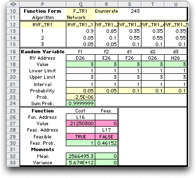
The form is constructed as below. For the example,
we have placed it immediately to the right of the transportation
model. The five distributions are at the top of the form. Rows
16 through 24 are used by the enumeration process. Rows 25
through 33 define the functions to be evaluated and the results.
This form is set to find the expected cost and the probability
that the given value of x results in a feasible
solution.
To find the expected value of the transportation
solution we enumerate all possible values for the random variables.
Since each random variable has three values there are 3 to
the fifth power, or 243, combinations. This is accomplished
by selecting the Moments command
from the menu. The program runs through all combinations of
the random variables. The values for each combination are placed
on the transportation model and the model is solved with the Network add-in.
The Random Variables add-in then combines all these
results to find the expected cost and the probability of a
feasible solution. These are in Q32 and R28 respectively.
|
| |
|
| |
For the example we have:
|
| |
The same process is used to compute several other solutions
below. For each we place the values of x in
cells K11 and K12. Then we choose Moments from the
menu to compute the expected value.
|
Expected Value Strategy |
| |
For this solution, we replace the random variables with
their expected values. The model then becomes a deterministic
linear program. The expected values of the random variables
are computed with the usual formulas for discrete random
variables.
Expected Value Model

|
The expected value solution places capacity only at generator
2. The expected cost and feasibility probability are computed
with the Moments command.
|
Scenario Analysis
Strategy |
| |
For this strategy we solve the
problem with a wait-and-see approach
and record the solution vector for each combination of the
random variables. This involves the solution of 243 separate
transportation models. We then combine the solutions by weighing
each solution by the probability of the combination and summing
the results. That solution is then used for the first-stage
decisions.
|
Summary |
| |
Comparing the three solutions on this page we note that the
optimum solution and the nearly optimum L-Shaped solution
dominate the other two in that it has a smaller cost and a
greater probability
of
feasibility.
Solution
|
Objective Value
|
Feasibility Probability
|
| Optimum Solution |
1,927,687
|
0.902
|
| L-Shaped Algorithm Solution |
1,927,689
|
0.902
|
| Expected Value Strategy |
2,433,951
|
0.700
|
| Scenario Analysis Strategy |
2,629,301
|
0.466
|
|


